
Land Cover Classification and Accuracy Assessment
with optical data
using Random Forest Classifier
in Google Earth Engine
This tutorial will teach you how to create a land cover map and assess its accuracy in Google Earth Engine. You will work with optical data from Landsat 8, starting with loading the analysis-ready data for the region of interest and preparing it for classification. You will then utilize a supervised classification algorithm, Random Forest, to generate a land cover map based on optical information. You will assess the accuracy of the classification with error matrices and kappa statistics based on the test data, which are the pixels randomly selected among the training set.

SDG 2: Zero Hunger Relevance
Land-use and land-cover maps are essential tools for decision-makers in formulating policies for sustainable development. Owing to continuous data acquisition at repetitive intervals, EO data enables the evaluation of the static (types, area, and arrangement) and dynamic attributes of land cover (rates of change).
Land cover maps can be utilized for Zero Hunger targets 2-3, 2-4, and 2-C by providing information on the distribution of land cover types, their extent, and their change in time. Moreover, they can reliably and consistently contribute to the monitoring, and reporting of the SDG indicator: 2.4.1 Proportion of agricultural area under productive and sustainable agriculture.
For more detail check the documentation ‘Specifications of land cover datasets for SDG indicator monitoring’ from (Carter & Herold, 2019) on:
Explore below the SDG 2: Zero Hunger relevance of applications related to
- Crop & Grazing Land Monitoring – Agriculture & Livestock
- Forest & Water Monitoring – Forestry & Agroforestry – Fishery & Aquaculture
- Environmental Monitoring – Agriculture & Livestock – Forestry & Agroforestry – Fishery & Aquaculture
Source Tutorial
This tutorial is part of the NASA Applied Remote Sensing Training Program (ARSET). Original creators: Zach Bengtsson, Britnay Beaudry, Juan Torres-Pérez, & Amber McCullum
The original content can be found at:
NASA-ARSET Training: Using Google Earth Engine for Land Monitoring Applications
Part 2: Land Cover Classification and Accuracy Assessment in Google Earth Engine

By loading the video, you agree to YouTube’s privacy policy.
Learn more
On ARSET’s training site, you will find a video providing step-by-step instructions and explanations for the tutorial. The first part of the video provides the relevant background information. It explains what classification is, how it works, what types of classification methods there are, and in particular how Random Forest works. You will also find the presentation slides and Q&A Transcript from the course.
Note that there are some updates in the version provided here. For instance, USGS Landsat 8 Surface Reflectance Tier 1 data is deprecated and replaced by USGS Landsat 8 Level 2, Collection 2, Tier 1. The cloud masking function is adapted to the new dataset (Stack Exchange, n.d.).
The Data, Processing Tools and Region of Interest
Data sets
You will load the analysis-ready data directly on Google Earth Engine. The training data and shape file are also provided with the code.
| EO data | |
| Optical Data: Landsat 8 Analysis-ready data: USGS Landsat 8 Level 2, Collection 2, Tier 1 Provider: USGS | – 19 Bands: Surface reflectance for different wavelengths (7), and a variety of additional bands – Resolution: 30 m – Analysis-ready data: Surface reflectance image – ‘Estimation of the fraction of incoming solar radiation that is reflected from Earth’s surface to the Landsat sensor by correcting for the artifacts from the atmosphere, illumination, and viewing geometry.’ |
| Training data | You will import the available training data directly on GEE for the land cover classes of cultivated, coniferous, mixed forest, deciduous, and water. |
| Shapefile | The shape file is available as GEE assets (CCMaine). |
Processing Software/Platform
Google Earth Engine (GEE) is used for the processing of the EO data.
- Go to https://code.earthengine.google.com and create an account if you don‘t already have one.
- You will find the here the Earth Engine Code Editor Guide
Region of Interest
The region of interest is located in Cumberland County, Maine, USA.
- training data is available for the classes:
cultivated, coniferous, mixed forest, deciduous, water
Processing Steps
Explore below the interactive flow chart!
Step-by-step instructions
Download the instruction file:
The GEE code
The entire code for the tutorial is already available. Click on the following button for the code in GEE with imported training data and shape file (see the import entries at the top of the code).
Go to the GEE code:
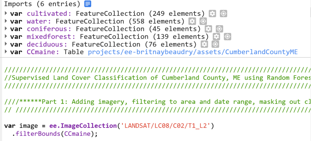
Part 1: Adding imagery, filtering to area and date range, masking out clouds, and making a composite
/////////////////////////////////////////////////////////////////////////////////////
//Supervised Land Cover Classification of Cumberland County, ME using Random Forest//
/////////////////////////////////////////////////////////////////////////////////////

////******Part 1: Adding imagery, filtering to area and date range, masking out clouds, and making a composite.******
// ////////////////////////////////////////////////////////////////////////////////

var image = ee.ImageCollection('LANDSAT/LC08/C02/T1_L2')
  .filterBounds(CCmaine);

 Map.centerObject(CCmaine, 7);
 Map.addLayer(image, {bands: ['SR_B4', 'SR_B3', 'SR_B2'], min: 0, max: 0.2}, 'L8');


// // Function that scales and masks Landsat 8 (C2) surface reflectance images.

function maskL8sr(image) {
  // Develop masks for unwanted pixels (fill, cloud, cloud shadow).
  var qaMask = image.select('QA_PIXEL').bitwiseAnd(parseInt('11111', 2)).eq(0);
  var saturationMask = image.select('QA_RADSAT').eq(0);

  // Apply the scaling factors to the appropriate bands.
  var getFactorImg = function(factorNames) {
    var factorList = image.toDictionary().select(factorNames).values();
    return ee.Image.constant(factorList);
  };
  var scaleImg = getFactorImg([
    'REFLECTANCE_MULT_BAND_.|TEMPERATURE_MULT_BAND_ST_B10']);
  var offsetImg = getFactorImg([
    'REFLECTANCE_ADD_BAND_.|TEMPERATURE_ADD_BAND_ST_B10']);
  var scaled = image.select('SR_B.|ST_B10').multiply(scaleImg).add(offsetImg);

  // Replace original bands with scaled bands and apply masks.
  return image.addBands(scaled, null, true)
    .updateMask(qaMask).updateMask(saturationMask);
}

//Filter imagery for 2020 and 2021 summer date ranges.
//Create joint filter and apply it to Image Collection.
var sum20 = ee.Filter.date('2020-06-01','2020-09-30');
var sum21 = ee.Filter.date('2021-06-01','2021-09-30');

var SumFilter = ee.Filter.or(sum20, sum21);

var allsum = image.filter(SumFilter);

//--------------------------------------------------------------------

//Make a Composite: Apply the cloud mask function, use the median reducer,
//and clip the composite to our area of interest
var composite = allsum
              .map(maskL8sr)
              .median()
              .clip(CCmaine);


//Display the Composite

Map.addLayer(composite, {bands: ['SR_B4','SR_B3','SR_B2'],min: 0, max: 0.3},'Cumberland Color Image');
Part 2: Add Developed Land Data to determine the impervious surfaces
// ////******Part 2: Add Developed Land Data******
// ///////////////////////////////////////////////

//Add the impervious surface layer
var impervious = ee.ImageCollection('USGS/NLCD_RELEASES/2019_REL/NLCD')
                .filterDate('2019-01-01', '2020-01-01')
                .filterBounds(CCmaine)
                .select('impervious')
                .map(function(image){return image.clip(CCmaine)});

//Reduce the image collection to
var reduced = impervious.reduce('median');

//Mask out the zero values in the data
var masked = reduced.selfMask();
Part 3: Prepare for the Random Forest model
////******Part 3: Prepare for the Random Forest model******
////////////////////////////////////////////////

// In this example, we use land cover classes:
// 1-100 = Percent Impervious Surfaces
// 101 = coniferous
// 102 = mixed forest
// 103 = deciduous
// 104 = cultivated
// 105 = water
// 106 = cloud (masked out)

//Merge land cover classifications into one feature class
var newfc = coniferous.merge(mixedforest).merge(deciduous).merge(cultivated).merge(water);

//Specify the bands to use in the prediction.
var bands = ['SR_B3', 'SR_B4', 'SR_B5', 'SR_B6', 'SR_B7'];

//Make training data by 'overlaying' the points on the image.
var points = composite.select(bands).sampleRegions({
  collection: newfc,
  properties: ['landcover'],
  scale: 30
}).randomColumn();

//Randomly split the samples to set some aside for testing the model's accuracy
//using the "random" column. Roughly 80% for training, 20% for testing.
var split = 0.8;
var training = points.filter(ee.Filter.lt('random', split));
var testing = points.filter(ee.Filter.gte('random', split));

//Print these variables to see how much training and testing data you are using
print('Samples n =', points.aggregate_count('.all'));
print('Training n =', training.aggregate_count('.all'));
print('Testing n =', testing.aggregate_count('.all'));
Part 4: Random Forest Classification and Accuracy Assessments
//Part 4: Random Forest Classification and Accuracy Assessments
//////////////////////////////////////////////////////////////////////////

//Run the RF model using 300 trees and 5 randomly selected predictors per split ("(300,5)").
//Train using bands and land cover property and pull the land cover property from classes
var classifier = ee.Classifier.smileRandomForest(300,5).train({
features: training,
classProperty: 'landcover',
inputProperties: bands
});

//Test the accuracy of the model
////////////////////////////////////////
//Print Confusion Matrix and Overall Accuracy
var confusionMatrix = classifier.confusionMatrix();
print('Confusion matrix: ', confusionMatrix);
print('Training Overall Accuracy: ', confusionMatrix.accuracy());
var kappa = confusionMatrix.kappa();
print('Training Kappa', kappa);

var validation = testing.classify(classifier);
var testAccuracy = validation.errorMatrix('landcover', 'classification');
print('Validation Error Matrix RF: ', testAccuracy);
print('Validation Overall Accuracy RF: ', testAccuracy.accuracy());
var kappa1 = testAccuracy.kappa();
print('Validation Kappa', kappa1);

//Apply the trained classifier to the image
var classified = composite.select(bands).classify(classifier);
Part 5:Create a legend
////******Part 5:Create a legend******
//////////////////////////////////////

//Set position of panel
var legend = ui.Panel({
  style: {
    position: 'bottom-left',
    padding: '8px 15px'
  }
});

//Create legend title
var legendTitle = ui.Label({
  value: 'Classification Legend',
  style: {
    fontWeight: 'bold',
    fontSize: '18px',
    margin: '0 0 4px 0',
    padding: '0'
    }
});

//Add the title to the panel
legend.add(legendTitle);

//Create and style 1 row of the legend.
var makeRow = function(color, name) {

      var colorBox = ui.Label({
        style: {
          backgroundColor: '#' + color,
          padding: '8px',
          margin: '0 0 4px 0'
        }
      });

      var description = ui.Label({
        value: name,
        style: {margin: '0 0 4px 6px'}
      });

      return ui.Panel({
        widgets: [colorBox, description],
        layout: ui.Panel.Layout.Flow('horizontal')
      });
};

//Identify palette with the legend colors
var palette =['CCADE0', 'A052D3', '633581', '18620f', '3B953B','89CD89', 'EFE028', '0b4a8b'];

//Identify names within the legend
var names = ['Low Density Development','Mid Density Development','High Density Development',
            'Coniferous','Mixed Forest','Deciduous','Cultivated','Water'];

//Add color and names
for (var i = 0; i < 8; i++) {
  legend.add(makeRow(palette[i], names[i]));
  }

//Add legend to map
Map.add(legend);
Part 6: Display the Final Land Cover Classification and Provide Export Options
////******Part 6: Display the Final Land Cover Classification and Provide Export Options******
//////////////////////////////////////////////////////////////////////////////////////////////

//Create palette for the final land cover map classifications
var urbanPalette =
'<RasterSymbolizer>' +
' <ColorMap  type="intervals">' +
    '<ColorMapEntry color="#CCADE0" quantity="22" label="Low Density Development"/>' +
    '<ColorMapEntry color="#A052D3" quantity="56" label="Mid Density Development"/>' +
    '<ColorMapEntry color="#633581" quantity="100" label="High Density Development"/>' +
    '<ColorMapEntry color="#18620f" quantity="101" label="Coniferous"/>' +
    '<ColorMapEntry color="#3B953B" quantity="102" label="Mixed Forest"/>' +
    '<ColorMapEntry color="#89CD89" quantity="103" label="Deciduous"/>' +
    '<ColorMapEntry color="#EFE028" quantity="104" label="Cultivated"/>' +
    '<ColorMapEntry color="#0b4a8b" quantity="105" label="Water"/>' +
  '</ColorMap>' +
'</RasterSymbolizer>';

//Mask out impervious surfaces
var finalmap = classified.blend(masked);

//Add final map to the display
Map.addLayer(finalmap.sldStyle(urbanPalette), {}, "Land Classification");

//Center the map for display
Map.setCenter(-70.3322, 43.8398, 10);


Export.image.toDrive({
  image: finalmap.sldStyle(urbanPalette),
  description: 'imageToCOGeoTifffinal',
  region: CCmaine,
  fileFormat: 'GeoTIFF',
  formatOptions: {
    cloudOptimized: true
  }
});
Training Points
// In this example, we use land cover classes:
1-100 = Percent Impervious Surfaces
101 = coniferous
102 = mixed forest
103 = deciduous
104 = cultivated
105 = water
Below, you will find example code for these land cover classes. Please note that each training point is defined by its coordinates and land cover class value as assigned above.
Click on the blue page icon at top of the code editor to see the scripts of the imports.
 coniferous = /* color: #18620f */ee.FeatureCollection(
        [ee.Feature(
            ee.Geometry.Point([-70.19540920695977, 43.67651867869241]),
            {
              "landcover": 101,
              "system:index": "0"
            }),

  mixedforest = /* color: #5c9b00 */ee.FeatureCollection(
        [ee.Feature(
            ee.Geometry.Point([-70.43929592817392, 43.874845545095646]),
            {
              "landcover": 102,
              "system:index": "0"
            }),

   deciduous = /* color: #c3f7d3 */ee.FeatureCollection(
        [ee.Feature(
            ee.Geometry.Point([-70.08666895174571, 43.71533568237313]),
            {
              "landcover": 103,
              "system:index": "0"
            }),

cultivated = /* color: #f6ffba */ee.FeatureCollection(
        [ee.Feature(
            ee.Geometry.Point([-69.93993211396594, 43.901248411541246]),
            {
              "landcover": 104,
              "system:index": "0"
               })]),

  water = /* color: #0b4a8b */ee.FeatureCollection(
        [ee.Feature(
            ee.Geometry.Point([-70.62777422540455, 43.98994370954868]),
            {
              "landcover": 105,
              "system:index": "0"
         })]),

  CCmaine = ee.FeatureCollection("projects/ee-britnaybeaudry/assets/CumberlandCountyME");
Infoboxes
Explore the infoboxes below to gain insights into the EO data, tools, and techniques utilized in the hands-on tutorial.
You can find all the Towards Zero Hunger infoboxes in the module:

Techniques
Click on the three-dot icon below the slides for the full-screen option.
Data
Click on the three-dot icon below the slides for the full-screen option.
Tools
Click on the three-dot icon below the slides for the full-screen option.
Credit
This topic was created with the help of learning materials that were kindly provided by:
- NASA Applied Remote Sensing Training Program (ARSET): Bengtsson, Z.; Beaudry, B.; Torres-Pérez, J.; McCullum, A. (2021). Using Google Earth Engine for Land Monitoring Applications.
Sources & further reading
- Bengtsson, Z., Beaudry, B., Torres-Pérez, J., & McCullum, A. (2021). Using Google Earth Engine for Land Monitoring Applications. NASA Applied Remote Sensing Training Program (ARSET).
https://appliedsciences.nasa.gov/join-mission/training/english/arset-using-google-earth-engine-land-monitoring-applications - Carter, S., & Herold, M. (2019). Specifications of land cover datasets for SDG indicator monitoring. https://ggim.un.org/documents/Paper_Land_cover_datasets_for_SDGs.pdf
- Stack Exchange. (n.d.). How to make a cloud-free composite for Landsat 8 Collection 2 surface reflectance in Earth Engine. Retrieved May 15, 2023, from
https://gis.stackexchange.com/questions/425159/how-to-make-a-cloud-free-composite-for-landsat-8-collection-2-surface-reflectanc
Tell us which practical applications in the context of Zero Hunger and EO you would like to learn about in the future!
Click to navigate to the Towards Zero Hunger course page or Hand-on Tutorials page


Responses