Land Cover Classification
with optical & radar data
using Random Forest Classifier
in Google Earth Engine
With this tutorial, you will learn how to create a Land Cover Map using both SAR and Optical data in Google Earth Engine. You will work with optical data from Landsat 8 and SAR data from Sentinel-1. Start with loading and preparing the data set for the classification. You will then utilize a supervised classification algorithm, Random Forest, to generate a Land Cover Map. In the final step, you will assess the accuracy of the classification with error (confusion) matrices.
Benefits of using both Radar and optical data (Podest et all. 2020)]:
- Improved land cover classification
- Ability to provide a more detailed characterization of land changes
- Broad classes of land cover and change (optical)
- Land surface roughness and soil moisture (radar)
- Ability to monitor vegetation health more accurately for agricultural purposes, forest disturbances, and land degradation
- NDVI and/or EVI (optical)
- Plant structure and volume (radar)

SDG 2: Zero Hunger Relevance
Land-use and land-cover maps are essential tools for decision-makers in formulating policies for sustainable development. Owing to continuous data acquisition at repetitive intervals, EO data enables the evaluation of the static (types, area, and arrangement) and dynamic attributes of land cover (rates of change).
Land cover maps can be utilized for Zero Hunger targets 2-3, 2-4, and 2-C by providing information on the distribution of land cover types, their extent, and their change in time. Moreover, they can reliably and consistently contribute to the monitoring, and reporting of the SDG indicator: 2.4.1 Proportion of agricultural area under productive and sustainable agriculture.
For more detail check the documentation ‘Specifications of land cover datasets for SDG indicator monitoring’ from (Carter & Herold, 2019) on:
Explore below the SDG 2: Zero Hunger relevance of applications related to
- Crop & Grazing Land Monitoring – Agriculture & Livestock
- Forest & Water Monitoring – Forestry & Agroforestry – Fishery & Aquaculture
- Environmental Monitoring – Agriculture & Livestock – Forestry & Agroforestry – Fishery & Aquaculture
Source Tutorial
This tutorial is part of the NASA Applied Remote Sensing Training Program (ARSET). Original creators: Erika Podest, Amber McCullum, Juan Luis Torres Perez & Sean McCartney
The original content can be found at:
NASA-ARSET Training: Forest Mapping and Monitoring with SAR Data
Part 2: Land Cover Classification with Radar and Optical Data

By loading the video, you agree to YouTube’s privacy policy.
Learn more
On ARSET’s training site, you will find a video providing step-by-step instructions and explanations for the tutorial. The first part of the video provides the relevant background information. It provides brief information on attributes of optical and SAR data that are relevant for forest monitoring, and explains image classification with Random Forest. You will also find the presentation slides and Q&A Transcript from the course.
Note that there are some updates in the version provided here. For instance, USGS Landsat 8 Surface Reflectance Tier 1 data is deprecated and replaced by USGS Landsat 8 Level 2, Collection 2, Tier 1. The cloud masking function is adapted to the new dataset (Stack Exchange, n.d.).
The Data, Processing Tools and Region of Interest
Data sets
You will load the analysis-ready data directly on Google Earth Engine. The training data and shape file are also provided with the code.
| EO data | Data Characteristics |
| SAR data: Sentinel- 1 Analysis-ready data: C-band Synthetic Aperture Radar Ground Range Detected, log scaling Provider: European Union/ESA/Copernicus | – C-band SAR – 4 Bands: HH-VV-VH-HV polarizations – Resolution: 10 m – Pixel values are in dB – Descending – Analysis-ready data: calibrated, ortho-corrected GRD product pre-processing details |
| Optical data: Landsat 8 Analysis-ready data: USGS Landsat 8 Level 2, Collection 2, Tier 1 Provider: USGS | – 19 Bands: Surface reflectance for different wavelengths (7), and a variety of additional bands – Resolution: 30 m – Analysis-ready data: Surface reflectance image – ‘Estimation of the fraction of incoming solar radiation that is reflected from Earth’s surface to the Landsat sensor by correcting for the artefacts from the atmosphere, illumination, and viewing geometry.’ |
Processing Software/Platform
Google Earth Engine (GEE) is used for the processing of the EO data.
- Go to https://code.earthengine.google.com and create an account if you don‘t already have one.
- You will find here the Earth Engine Code Editor Guide
Region of Interest
The region of interest is located in Rondônia, Brazil
- Rondônia is one of the most biodiverse areas of the Amazon, with a wide range of habitat types and topography. However, the area undergoes intense and rapid deforestation due to the conversion of forested areas into pasture and croplands.
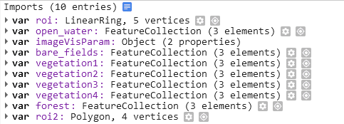
- 7 land cover classes are defined, these are: Open water, bare fields, vegetation1, vegetation2, vegetation3, vegetation4, forest
The types are defined based on the backscatter values: lowest (water) to highest (forest) backscatter
Processing Steps
Explore below the interactive flow chart!
Step-by-step instructions
Download the instruction file:
The GEE code
The entire code for the tutorial is already available. Click on the following button for the code in GEE with imported training data and shape file (see the import entries at the top of the code).
Go to the GEE code:
Load the EO Data
//-------------------------------------------------------------------
// Load the SAR data
//-------------------------------------------------------------------
// Load Sentinel-1 C-band SAR Ground Range collection (log scale, VV,descending)
var collectionVV = ee.ImageCollection('COPERNICUS/S1_GRD')
.filter(ee.Filter.eq('instrumentMode', 'IW'))
.filter(ee.Filter.listContains('transmitterReceiverPolarisation', 'VV'))
.filter(ee.Filter.eq('orbitProperties_pass', 'DESCENDING'))
.filterMetadata('resolution_meters', 'equals' , 10)
.filterBounds(roi)
.select('VV');
print(collectionVV, 'Collection VV');

// Load Sentinel-1 C-band SAR Ground Range collection (log scale, VH, descending)
var collectionVH = ee.ImageCollection('COPERNICUS/S1_GRD')
.filter(ee.Filter.eq('instrumentMode', 'IW'))
.filter(ee.Filter.listContains('transmitterReceiverPolarisation', 'VH'))
.filter(ee.Filter.eq('orbitProperties_pass', 'DESCENDING'))
.filterMetadata('resolution_meters', 'equals' , 10)
.filterBounds(roi)
.select('VH');
print(collectionVH, 'Collection VH');

//Filter by date
var SARVV = collectionVV.filterDate('2019-08-01', '2019-08-10').mosaic();
var SARVH = collectionVH.filterDate('2019-08-01', '2019-08-10').mosaic();

// Add the SAR images to "layers" in order to display them
Map.centerObject(roi, 7);
Map.addLayer(SARVV, {min:-15,max:0}, 'SAR VV', 0);
Map.addLayer(SARVH, {min:-25,max:0}, 'SAR VH', 0);


//-------------------------------------------------------------------
// Load the optical data
//-------------------------------------------------------------------
// Function to cloud mask from the pixel QA band of Landsat 8 SR data.
function maskL8sr(image) {
// Bits 3 and 5 are cloud shadows and clouds, respectively.
var cloudShadowBitMask = 1 << 3;
var cloudsBitMask = 1 << 5;
// Get the pixel QA band.
var qa = image.select('pixel_qa');
// Both flags should be set to zero, indicating clear conditions.
var mask = qa.bitwiseAnd(cloudShadowBitMask).eq(0)
.and(qa.bitwiseAnd(cloudsBitMask).eq(0));
// Return the masked image, scaled to reflectance, without the QA bands.
return image.updateMask(mask).divide(10000)
.select("B[0-9]*")
.copyProperties(image, ["system:time_start"]);
}

// Extract the images from the Landsat8 collection
var collectionl8 = ee.ImageCollection('LANDSAT/LC08/C01/T1_SR')
.filterDate('2019-08-01', '2019-08-10')
.filterBounds(roi)
.map(maskL8sr);
print(collectionl8, 'Landsat');
Generate NDVI images (Landsat-8) and apply speckle filter (Sentinel-1)
//-------------------------------------------------------------------
// Generate NDVI images from the Landsat 8 data
//-------------------------------------------------------------------
//Calculate NDVI and create an image that contains all Landsat 8 bands and NDVI
var comp = collectionl8.mean();
var ndvi = comp.normalizedDifference(['B5', 'B4']).rename('NDVI');
var composite = ee.Image.cat(comp,ndvi);

// Add images to layers in order to display them
Map.centerObject(roi, 7);
Map.addLayer(composite, {bands: ['B4', 'B3', 'B2'], min: 0.1, max: 0.2}, 'Optical');
//change 0 to 0.1 upwards


//-------------------------------------------------------------------
// Apply speckle filter over the SAR data
//-------------------------------------------------------------------
//Apply filter to reduce speckle
var SMOOTHING_RADIUS = 50;
var SARVV_filtered = SARVV.focal_mean(SMOOTHING_RADIUS, 'circle', 'meters');
var SARVH_filtered = SARVH.focal_mean(SMOOTHING_RADIUS, 'circle', 'meters');

//Display the SAR filtered images
Map.addLayer(SARVV_filtered, {min:-15,max:0}, 'SAR VV Filtered',0);
Map.addLayer(SARVH_filtered, {min:-25,max:0}, 'SAR VH Filtered',0);
Collect training data for the supervised classification and classify with Sentinel-1
The first step in performing supervised classification is to collect training data to ‘train’ the classifier. This requires collecting representative samples of backscatter for each land cover class of interest. This involves:
- Collecting a representative sample of polygons for each class
- Importing the geometry as FeatureCollection
- Use the Add property to set a value to the class and assign a color for display.
After collection of the training points, you will see the entries on top of the code under imports.
The next step is to merge the classes into a single collection, define the bands to train the data, train the classifier and run the classifier.
//-------------------------------------------------------------------
// Collect training data for supervised classification with Random Forest
//-------------------------------------------------------------------
//Merge Feature Collections
var newfc = open_water.merge(bare_fields).merge(vegetation1).merge(vegetation2).merge(vegetation3).merge(vegetation4).merge(forest);

//Define the SAR bands to train your data
var final = ee.Image.cat(SARVV_filtered,SARVH_filtered);
var bands = ['VH','VV'];
var training = final.select(bands).sampleRegions({
collection: newfc,
properties: ['landcover'],
scale: 30 });

//Train the classifier
var classifier = ee.Classifier.smileCart().train({
features: training,
classProperty: 'landcover',
inputProperties: bands
});

//Run the Classifier
var classified = final.select(bands).classify(classifier);

//Display the Classification
Map.addLayer(classified,
{min: 1, max: 7, palette: ['1667fa', 'c9270d', 'cf7b68', 'ee9a1c', '146d0e', '04bd23', '37fe05']},
'SAR Classification');
Classify the Optical image
//-------------------------------------------------------------------
// Classify the Optical image: Supervised Classification with Random Forest
//-------------------------------------------------------------------
//Define the Landsat bands to train your data
var bandsl8 = ['B1', 'B2', 'B3', 'B4', 'B5', 'B6', 'B7', 'B10', 'B11', 'NDVI' ];
//var bandsl8 = ['NDVI' ];
var trainingl8 = composite.select(bandsl8).sampleRegions({
collection: newfc,
properties: ['landcover'],
scale: 30
});

//Train the classifier
var classifierl8 = ee.Classifier.smileCart().train({
features: trainingl8,
classProperty: 'landcover',
inputProperties: bandsl8
});

//Run the Classifier
var classifiedl8 = composite.select(bandsl8).classify(classifierl8);

//Display the Classification
Map.addLayer(classifiedl8,
{min: 1, max: 7, palette: ['1667fa', 'c9270d', 'cf7b68', 'ee9a1c', '146d0e', '04bd23', '37fe05']},
'Optical Classification');
Assess the Accuracy
//-------------------------------------------------------------------
// Assess the Accuracy of SAR-based classification
//-------------------------------------------------------------------
// Create a confusion matrix representing resubstitution accuracy.
print('RF- SAR error matrix: ', classifier.confusionMatrix());
print('RF- SAR accuracy: ', classifier.confusionMatrix().accuracy());

//-------------------------------------------------------------------
// Assess the Accuracy of Optical based classification
//-------------------------------------------------------------------
// Create a confusion matrix representing resubstitution accuracy.
print('RF-L8 error matrix: ', classifierl8.confusionMatrix());
print('RF-L8 accuracy: ', classifierl8.confusionMatrix().accuracy());
Classification based on both Optical and SAR data & accuracy assessment
//-------------------------------------------------------------------
// Classification based on both Optical and SAR data
//-------------------------------------------------------------------
//Define both optical and SAR to train your data
var opt_sar = ee.Image.cat(composite, SARVV_filtered,SARVH_filtered);
var bands_opt_sar = ['VH','VV','B1', 'B2', 'B3', 'B4', 'B5', 'B6', 'B7', 'B10', 'B11', 'NDVI'];
var training_opt_sar = opt_sar.select(bands_opt_sar).sampleRegions({
collection: newfc,
properties: ['landcover'],
scale: 30 });

//Train the classifier
var classifier_opt_sar = ee.Classifier.smileCart().train({
features: training_opt_sar,
classProperty: 'landcover',
inputProperties: bands_opt_sar
});

//Run the classifier
var classifiedboth = opt_sar.select(bands_opt_sar).classify(classifier_opt_sar);

//Display the Classification
Map.addLayer(classifiedboth,
{min: 1, max: 7, palette: ['1667fa', 'c9270d', 'cf7b68', 'ee9a1c', '146d0e', '04bd23', '37fe05']},
'Optical/SAR Classification');

//-------------------------------------------------------------------
// Assess the Accuracy of both Optical and SAR-based classification
//-------------------------------------------------------------------
// Create a confusion matrix representing resubstitution accuracy.
print('RF-Opt/SAR error matrix: ', classifier_opt_sar.confusionMatrix());
print('RF-Opt/SAR accuracy: ', classifier_opt_sar.confusionMatrix().accuracy());
Export the classification as GeoTIFF
//-------------------------------------------------------------------
// Export the finished classification as GeoTIFF
//-------------------------------------------------------------------
// remap values in class to integer above so class 0 becomes free for noData pixels
var remap = ee.Image(classifiedboth)
 .remap([0,1,2,3,4,5,6,7], [1,2,3,4,5,6,7,8]);


print('remap',remap);
print(ee.List(classifiedboth));

// Get information about the bands as a list.
var bandNames = classifiedboth.bandNames();
print('Band names:', bandNames);  // ee.List of band names

// Get a list of all metadata properties.
var properties = classifiedboth.propertyNames();
print('Metadata properties:', properties);  // ee.List of metadata properties

var floatclass = classifiedboth.float;
print('flaot', floatclass);
 console.log(classifiedboth);


Export.image.toDrive({
image: classifiedboth.visualize({min: 1, max: 7, palette: ['1667fa', 'c9270d',  'cf7b68', 'ee9a1c',  '146d0e',  '04bd23',  '37fe05']}),
description: 'optical_SAR_classified',
scale: 500,
region: roi2,
fileFormat: 'GeoTIFF',
formatOptions: {
    cloudOptimized: true
  }
});

*/
Infoboxes
Explore the info-boxes below to gain insights into the EO data, tools, and techniques utilized in the hands-on tutorial.
You can find all the Towards Zero Hunger info-boxes in the module:

Techniques
Click on the three-dot icon below the slides for the full-screen option.
Data
Click on the three-dot icon below the slides for the full-screen option.
Tools
Click on the three-dot icon below the slides for the full-screen option.
Missions
Click on the three-dot icon below the slides for the full-screen option.
Credit
This topic was created with the help of learning materials that were kindly provided by:
- NASA Applied Remote Sensing Training Program (ARSET): Podest, E.; McCullum, A.; Torres-Pérez, J.; McCartney, S.; Siqueira, P.; Lei, Y.; Whelen, T.; Kraatz, S. (2020). Forest Mapping and Monitoring with SAR Data
Sources & further reading
- Podest, E.; McCullum, A.; Torres-Pérez, J.; McCartney, S.; Siqueira, P.; Lei, Y.; Whelen, T.; Kraatz, S. (2020). Forest Mapping and Monitoring with SAR Data. NASA Applied Remote Sensing Training Program (ARSET). https://appliedsciences.nasa.gov/join-mission/training/english/arset-forest-mapping-and-monitoring-sar-data
- Carter, S., & Herold, M. (2019). Specifications of land cover datasets for SDG indicator monitoring. https://ggim.un.org/documents/Paper_Land_cover_datasets_for_SDGs.pdf
- Stack Exchange. (n.d.). How to make a cloud-free composite for Landsat 8 Collection 2 surface reflectance in Earth Engine. Retrieved May 15, 2023, from
https://gis.stackexchange.com/questions/425159/how-to-make-a-cloud-free-composite-for-landsat-8-collection-2-surface-reflectanc
Tell us which practical applications in the context of Zero Hunger and EO you would like to learn about in the future!
Click to navigate to the Towards Zero Hunger course page or Hand-on Tutorials page


Responses