Classifying Commodities in GEE

Learning objectives of this tutorial
- Collect (training/validation) sample points in GEE
- Generate texture information from sentinel-2 spectral bands
- Apply the Random Forest classifier to identify commodities
- Determine the accuracy of your product
Prerequisites
- The tutorial of this lesson will be done in Google Earth Engine (GEE). If you are not familiar with GEE, link to the FAQ, and tutorials are provided.
- Image Classification could be useful for a recap of how to select for samples and the Random Forest classification method
Time estimate of this tutorial is 30 – 45 minutes. Note that running time will depend on the observation period and area of interest (aoi)
Introduction
This practical provides a basic workflow to map commodities using the spectral bands and texture information from Sentinel-2 data.
You will learn a series of GEE tools to:
- Collect training and validating dataset for a Random Forest model.
- Generate a cloud-free composite from Sentinel-2 imagery.
- Extract texture features from sentinel-2 cloud-free composite.
- Explore feature importance.
- Train and validate a Random Forest model.
- Generating a commodity map for your area of interest.
We will provide advanced reading material to discuss ways to improve the accuracy of the classification.
The skills and techniques you will lean are also applicable for other regions and other commodity types.
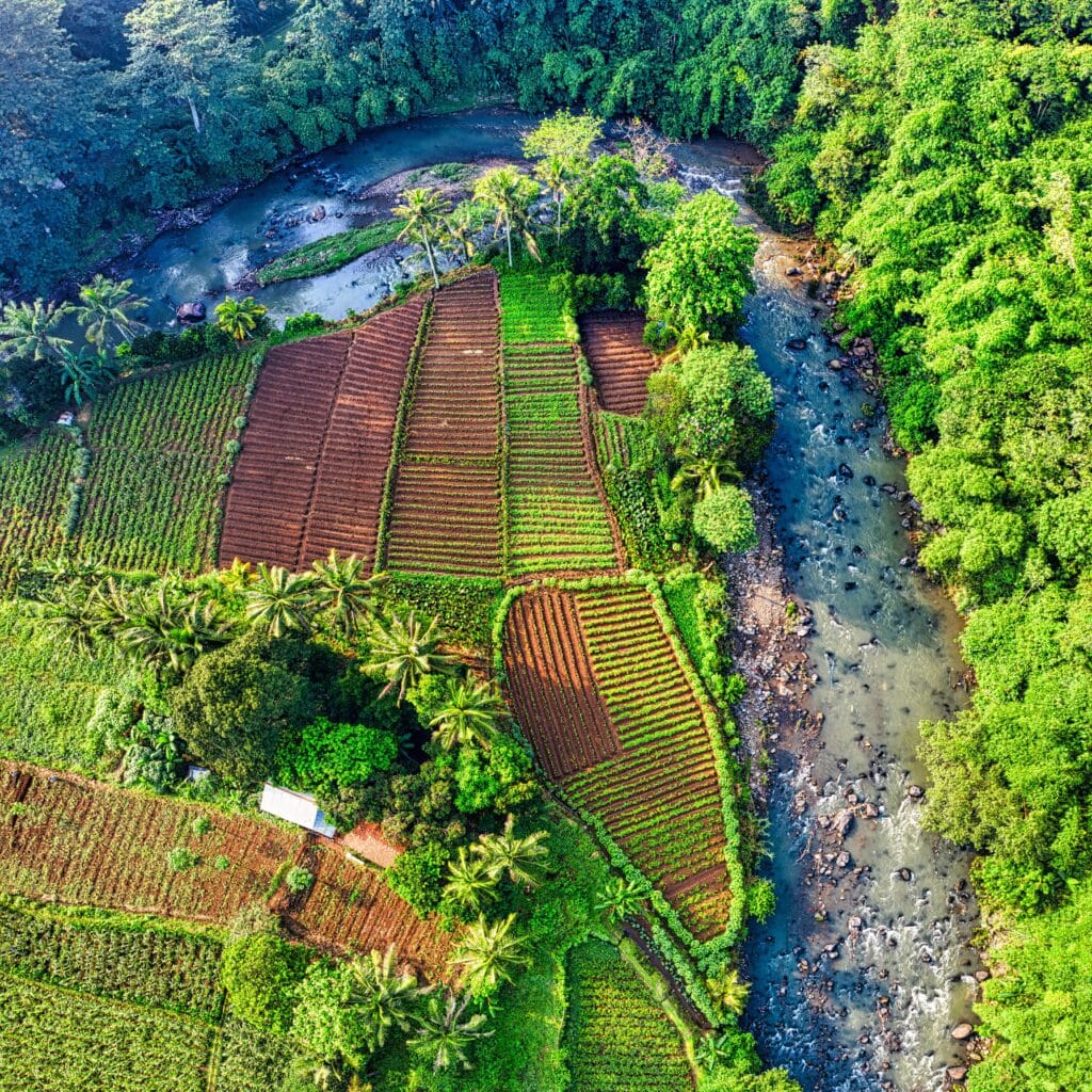
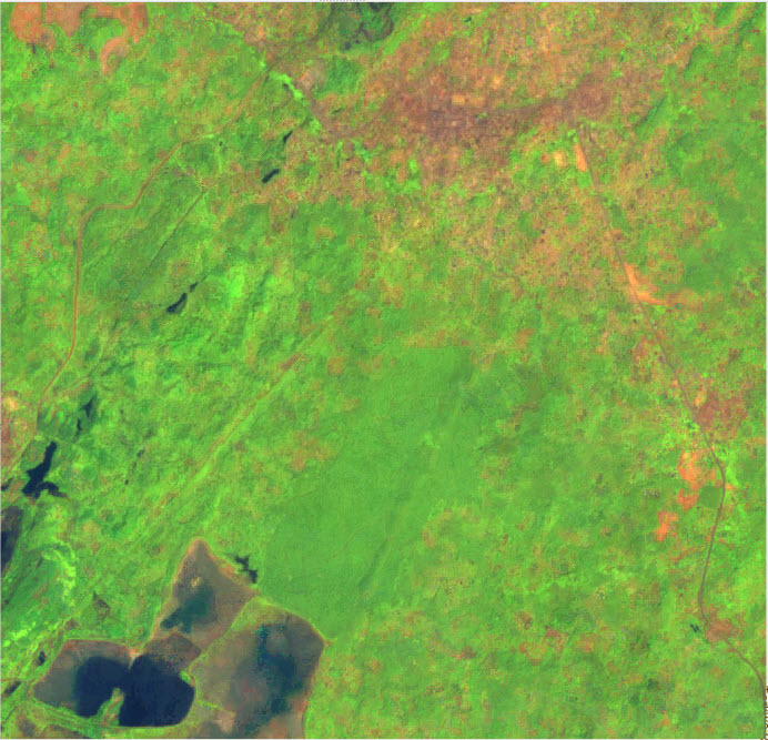
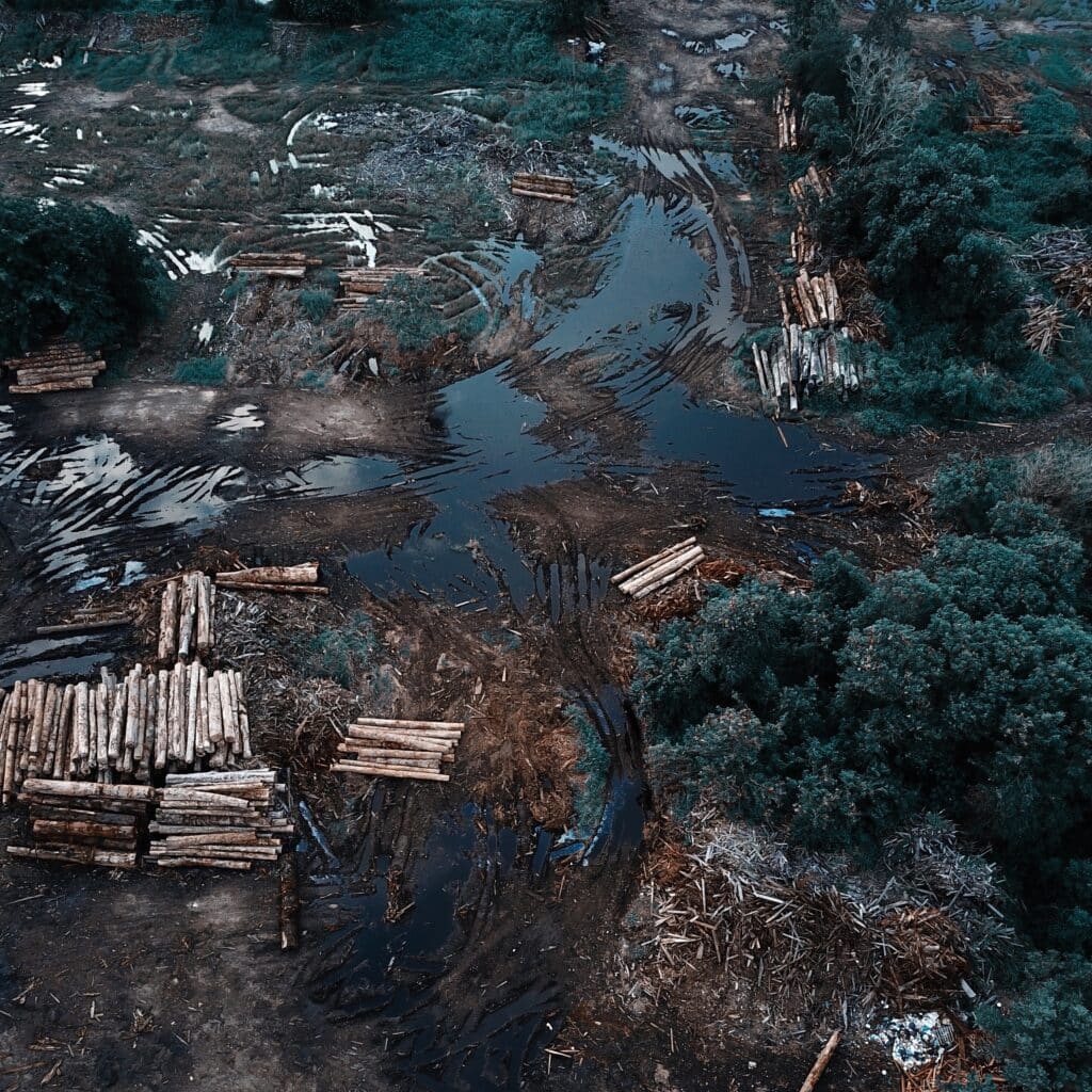
Study Area
The study area is around the district of Bogoso in Ghana, above you see a time lapse of the area in which a mine is being developed. In our analysis we will not be focusing on mining but rather on identifying palm, rubber, cocoa, and native forests.
Set up steps
You will need an active Google Earth Engine (GEE) account for this tutorial, if you haven’t signed up for an account yet, you can see the FAQ here and sign up here.
You will need to create a new script, throughout the tutorial you will be copying the code blocks from this page into your script and running them. If you need an introduction to the GEE environment, please take some time and review the documentation.
1. Imports (Close this accordion after copying the code)
In this step you will import the training polygons which will be used later on in the tutorial.
- Copy the following code into your new script, (Click the code twice to select all, then hold down Ctrl + C to copy.)
- Paste this code into your code editor, the code will be highlighted in orange,
- A pop-up asking whether you would like to convert ‘palm’, ‘cocoa’ … will appear, click “Convert” in the suggestion tooltip.
- The video below can help you with this step.
- Afterwards you can close this accordion item and move on to the next one, Setting Parameters and Import Functions.
var geometry =
/* color: #d63000 */
/* shown: false */
/* displayProperties: [
{
"type": "rectangle"
}
] */
ee.Geometry.Polygon(
[[[-2.0491730618606963, 5.583386879708488],
[-2.0491730618606963, 5.519700230146676],
[-1.9899498868118681, 5.519700230146676],
[-1.9899498868118681, 5.583386879708488]]], null, false),
palm =
/* color: #ca10ff */
/* shown: false */
ee.Geometry({
"type": "GeometryCollection",
"geometries": [
{
"type": "Polygon",
"coordinates": [
[
[
-2.0243250775467314,
5.538377661282055
],
[
-2.0245181965958037,
5.537672863266067
],
[
-2.0230805325638213,
5.5373525002536566
],
[
-2.0222007680069365,
5.537651505737301
],
[
-2.0211064267288603,
5.538527163783441
],
[
-2.0200764584671416,
5.539723182432645
],
[
-2.0206343579422392,
5.540812411595674
],
[
-2.022157852662698,
5.539936756936633
],
[
-2.023037618278536,
5.539520285779195
],
[
-2.0240461278091826,
5.53871938122964
]
]
],
"evenOdd": true
},
{
"type": "Polygon",
"coordinates": [
[
[
-2.015524319132762,
5.552392449856946
],
[
-2.0152453693952133,
5.552979766946103
],
[
-2.015256098231273,
5.553342835399386
],
[
-2.0164148125257064,
5.552541948807903
]
]
],
"geodesic": true,
"evenOdd": true
},
{
"type": "Polygon",
"coordinates": [
[
[
-2.0083795553740758,
5.5470962101593395
],
[
-2.008347368865897,
5.545868170598702
],
[
-2.007478333145072,
5.546103100103667
],
[
-2.007574892669608,
5.547299103405932
]
]
],
"geodesic": true,
"evenOdd": true
},
{
"type": "Polygon",
"coordinates": [
[
[
-2.0367866023680703,
5.573708325471087
],
[
-2.0373766883513467,
5.5725230539634145
],
[
-2.037441061367704,
5.571999825239415
],
[
-2.036496923794462,
5.5720425378057845
],
[
-2.0362072452208535,
5.573014247851498
]
]
],
"geodesic": true,
"evenOdd": true
},
{
"type": "Polygon",
"coordinates": [
[
[
-2.03066369404741,
5.570114003707728
],
[
-2.0310177456373757,
5.569238392601703
],
[
-2.0305510412687844,
5.56900347232686
],
[
-2.0301433454985207,
5.569921796503551
]
]
],
"geodesic": true,
"evenOdd": true
},
{
"type": "Polygon",
"coordinates": [
[
[
-2.022658084166078,
5.55968826940537
],
[
-2.0227653725266737,
5.559074263064314
],
[
-2.022159193289308,
5.558801964395033
],
[
-2.021885607969789,
5.5594159710201
],
[
-2.0225937111497205,
5.559698947770842
]
]
],
"geodesic": true,
"evenOdd": true
},
{
"type": "Polygon",
"coordinates": [
[
[
-2.030127498506602,
5.560585083943357
],
[
-2.02918336093336,
5.55977352883639
],
[
-2.0286469191303813,
5.559591996619846
],
[
-2.02867910563856,
5.560521013844022
],
[
-2.029751989244517,
5.560809329236114
]
]
],
"geodesic": true,
"evenOdd": true
},
{
"type": "Polygon",
"coordinates": [
[
[
-2.0301596850147807,
5.558566872463949
],
[
-2.029376479982432,
5.558961972610453
],
[
-2.0299665659657085,
5.5594745345675465
],
[
-2.0306853979816997,
5.558876545574227
]
]
],
"geodesic": true,
"evenOdd": true
},
{
"type": "Polygon",
"coordinates": [
[
[
-2.0153272308369585,
5.525922507484706
],
[
-2.015370146181197,
5.52452889943924
],
[
-2.0147532381077715,
5.524085720714665
],
[
-2.014195338632674,
5.525682230469429
]
]
],
"geodesic": true,
"evenOdd": true
},
{
"type": "Polygon",
"coordinates": [
[
[
-2.02152849807939,
5.525959883900534
],
[
-2.0208472169896075,
5.525655533017258
],
[
-2.0200479187031695,
5.527326791201868
],
[
-2.0206165470143267,
5.527727251727653
]
]
],
"geodesic": true,
"evenOdd": true
},
{
"type": "Polygon",
"coordinates": [
[
[
-1.9996691251670806,
5.537190980214035
],
[
-1.9997495914375274,
5.536641023154158
],
[
-1.999384811011502,
5.5364007504916595
],
[
-1.9992775226509063,
5.536667720110633
],
[
-1.998735716429898,
5.537164283281198
]
]
],
"geodesic": true,
"evenOdd": true
},
{
"type": "Polygon",
"coordinates": [
[
[
-2.042459590464394,
5.529663865246724
],
[
-2.042878015070717,
5.529044488211974
],
[
-2.042105538874428,
5.528756157302287
],
[
-2.041858775645058,
5.529386213552685
]
]
],
"geodesic": true,
"evenOdd": true
},
{
"type": "Polygon",
"coordinates": [
[
[
-2.048478498246553,
5.551110964960645
],
[
-2.048086895730379,
5.550699841756252
],
[
-2.047657742287996,
5.550956126384862
],
[
-2.048161997582796,
5.551345892377284
]
]
],
"geodesic": true,
"evenOdd": true
}
],
"coordinates": []
}),
other_veg =
/* color: #b0ef99 */
/* shown: false */
ee.Geometry({
"type": "GeometryCollection",
"geometries": [
{
"type": "Polygon",
"coordinates": [
[
[
-2.0296894955765166,
5.53414886057987
],
[
-2.029303257478372,
5.535857470566376
],
[
-2.0295178341995634,
5.536839919072578
],
[
-2.0301401066910185,
5.536370052599424
],
[
-2.0305692601334013,
5.535942900936078
],
[
-2.030698006166116,
5.534875020427432
]
]
],
"evenOdd": true
},
{
"type": "Polygon",
"coordinates": [
[
[
-2.030058519271958,
5.538820611004149
],
[
-2.029382602600205,
5.53887400471895
],
[
-2.028427736190903,
5.539375905402289
],
[
-2.0297473830262303,
5.5400700226660025
],
[
-2.030573503402817,
5.539461335263368
]
]
],
"geodesic": true,
"evenOdd": true
},
{
"type": "Polygon",
"coordinates": [
[
[
-2.02675403776561,
5.538649751084337
],
[
-2.026056663421738,
5.538745859795312
],
[
-2.025455848602402,
5.539375905402289
],
[
-2.0263248843232273,
5.539803054584166
]
]
],
"geodesic": true,
"evenOdd": true
},
{
"type": "Polygon",
"coordinates": [
[
[
-2.0341140193024754,
5.5363965312703485
],
[
-2.0332557124177097,
5.5368984340578775
],
[
-2.0330625933686375,
5.53792359587396
],
[
-2.0334059161225437,
5.537592554231914
],
[
-2.0340818327942967,
5.536727573582309
]
]
],
"geodesic": true,
"evenOdd": true
},
{
"type": "Polygon",
"coordinates": [
[
[
-2.028685228256333,
5.536407210057511
],
[
-2.0273655814210056,
5.537250833632723
],
[
-2.0276659888306736,
5.53768866311483
],
[
-2.0285993975678562,
5.537325585030675
]
]
],
"geodesic": true,
"evenOdd": true
},
{
"type": "Polygon",
"coordinates": [
[
[
-2.0320318052176023,
5.543688480705398
],
[
-2.031291515529492,
5.5444359861118615
],
[
-2.0320854493979,
5.544681594824497
]
]
],
"geodesic": true,
"evenOdd": true
},
{
"type": "Polygon",
"coordinates": [
[
[
-2.0111267005778943,
5.5496817201612
],
[
-2.011330548463026,
5.549740452166508
],
[
-2.0114432012416517,
5.5495268812100855
],
[
-2.011282268700758,
5.549340006559738
],
[
-2.0110730563975965,
5.549334667283144
],
[
-2.0108477508403455,
5.549558916858467
],
[
-2.0105795299388562,
5.549788505621047
],
[
-2.010407868561903,
5.550151576039874
],
[
-2.0105044280864393,
5.550322432630204
],
[
-2.010681453881422,
5.550130218962593
],
[
-2.010686818299452,
5.549932665961164
],
[
-2.0108745729304944,
5.549697737981415
]
]
],
"geodesic": true,
"evenOdd": true
},
{
"type": "Polygon",
"coordinates": [
[
[
-2.008426671729293,
5.563390222994177
],
[
-2.008378391967025,
5.563080552259149
],
[
-2.0077722127296593,
5.563497005968472
],
[
-2.0080887133934167,
5.563550397448348
]
]
],
"geodesic": true,
"evenOdd": true
},
{
"type": "Polygon",
"coordinates": [
[
[
-2.0103109602358193,
5.555657949948353
],
[
-2.0102895025637,
5.555417685029285
],
[
-2.0099327687647195,
5.555380310477516
],
[
-2.0101124767687173,
5.555593879312854
]
]
],
"geodesic": true,
"evenOdd": true
},
{
"type": "Polygon",
"coordinates": [
[
[
-2.0038869092777722,
5.535215196746221
],
[
-2.0045789192036145,
5.53462786198225
],
[
-2.0038600871876233,
5.534558449653419
],
[
-2.0033826539829724,
5.5347880442484625
],
[
-2.003640146048402,
5.535145784486331
]
]
],
"geodesic": true,
"evenOdd": true
}
],
"coordinates": []
}),
non_veg =
/* color: #8e958b */
/* shown: false */
ee.Geometry({
"type": "GeometryCollection",
"geometries": [
{
"type": "Polygon",
"coordinates": [
[
[
-2.034062719545473,
5.535067362136452
],
[
-2.0341056348897113,
5.532611230446625
],
[
-2.032238817415346,
5.532579193878923
],
[
-2.0323246481038226,
5.5333267133396475
],
[
-2.0327323438740863,
5.533679115043428
],
[
-2.033311701021303,
5.533849976399986
],
[
-2.0333546163655414,
5.534618851893559
],
[
-2.0334726335621967,
5.534843107057536
]
]
],
"evenOdd": true
},
{
"type": "Polygon",
"coordinates": [
[
[
-2.0320111674347996,
5.535317972774499
],
[
-2.0316142005005955,
5.534997608485784
],
[
-2.0312708777466892,
5.535446118441357
],
[
-2.031775133041489,
5.535755803688302
]
]
],
"geodesic": true,
"evenOdd": true
},
{
"type": "Polygon",
"coordinates": [
[
[
-2.026357070831406,
5.54146893344209
],
[
-2.025960103897202,
5.541319431685223
],
[
-2.02575625601207,
5.541693186006434
],
[
-2.0262175959626316,
5.541810651601389
]
]
],
"geodesic": true,
"evenOdd": true
},
{
"type": "Polygon",
"coordinates": [
[
[
-2.0333576363602757,
5.540502510702503
],
[
-2.032923118499863,
5.5409670345371405
],
[
-2.03300358477031,
5.541100518330095
],
[
-2.033518568901169,
5.540539886196976
]
]
],
"geodesic": true,
"evenOdd": true
},
{
"type": "Polygon",
"coordinates": [
[
[
-2.0255371546262158,
5.542215379810178
],
[
-2.025397679774228,
5.542300809253346
],
[
-2.0256229853520424,
5.542514382795242
],
[
-2.02588047735228,
5.542471668108005
]
]
],
"geodesic": true,
"evenOdd": true
},
{
"type": "Polygon",
"coordinates": [
[
[
-2.0200433367698767,
5.577217047624592
],
[
-2.0183803671806433,
5.580698080644219
],
[
-2.019506894966898,
5.580868928358677
],
[
-2.0208479994743445,
5.578114002893625
]
]
],
"geodesic": true,
"evenOdd": true
},
{
"type": "Polygon",
"coordinates": [
[
[
-2.031213464613122,
5.525654425572075
],
[
-2.029539766187829,
5.520870222710879
],
[
-2.0265356920911493,
5.524415662466248
],
[
-2.0262782000257196,
5.5278329337143335
]
]
],
"geodesic": true,
"evenOdd": true
},
{
"type": "Polygon",
"coordinates": [
[
[
-2.0402505148046757,
5.580269935107393
],
[
-2.040840600787952,
5.578860438534898
],
[
-2.039596055805042,
5.579832137292237
]
]
],
"geodesic": true,
"evenOdd": true
},
{
"type": "Polygon",
"coordinates": [
[
[
-2.004154763184647,
5.569121485140751
],
[
-2.004173538647751,
5.568526175506947
],
[
-2.0041386699305574,
5.568256550765862
],
[
-2.0036934232340853,
5.568291254947394
],
[
-2.003505668603043,
5.568857199772376
],
[
-2.003680012189011,
5.569364414010883
],
[
-2.003725609742264,
5.569815567360376
],
[
-2.00419499631987,
5.569551282304179
]
]
],
"geodesic": true,
"evenOdd": true
},
{
"type": "Polygon",
"coordinates": [
[
[
-1.9959318099335932,
5.540382787638842
],
[
-1.9958835301713251,
5.540009032488383
],
[
-1.9954811988190913,
5.54000369312739
],
[
-1.99551338532727,
5.54045753864056
]
]
],
"geodesic": true,
"evenOdd": true
},
{
"type": "Polygon",
"coordinates": [
[
[
-1.995835250409057,
5.54054296834522
],
[
-1.9956743178681635,
5.54066577352401
],
[
-1.9957762418107294,
5.541060885665174
],
[
-1.99601227620404,
5.540767221261155
]
]
],
"geodesic": true,
"evenOdd": true
},
{
"type": "Polygon",
"coordinates": [
[
[
-1.9962322173432612,
5.541365228620715
],
[
-1.99613834002774,
5.541520069713336
],
[
-1.9963153658227228,
5.541632195996443
],
[
-1.996411925347259,
5.5414346401500065
]
]
],
"geodesic": true,
"evenOdd": true
},
{
"type": "Polygon",
"coordinates": [
[
[
-1.9962933260657234,
5.5380161614648955
],
[
-1.9958749014594002,
5.537701138020443
],
[
-1.995703240082447,
5.537981455500434
],
[
-1.9957407910086555,
5.538227066897418
],
[
-1.9961163002707405,
5.5382671122241955
]
]
],
"geodesic": true,
"evenOdd": true
},
{
"type": "Polygon",
"coordinates": [
[
[
-1.9948921902882821,
5.545095000597148
],
[
-1.9947902663457162,
5.544625140691052
],
[
-1.9944737656819589,
5.5448066775173
],
[
-1.9945274098622567,
5.545132375800893
]
]
],
"geodesic": true,
"evenOdd": true
}
],
"coordinates": []
}),
open_forest =
/* color: #56af98 */
/* shown: false */
ee.Geometry.MultiPolygon(
[[[[-1.996642493340497, 5.549420123162319],
[-1.9966746798486756, 5.548896873897446],
[-1.9962133398981141, 5.548806106120566],
[-1.9960094920129823, 5.549350712572258]]],
[[[-1.9955266943903016, 5.549051713013987],
[-1.9946254721612977, 5.5484697312962235],
[-1.9942392340631532, 5.548902213177995],
[-1.995043896767621, 5.549564283592496],
[-1.995494507882123, 5.54938274823022]]],
[[[-1.9969858160944032, 5.5513649458561085],
[-1.9964869252176332, 5.5511780717883505],
[-1.9966049424142884, 5.551519784324517]]],
[[[-2.019125004583482, 5.575472628476249],
[-2.018577833944444, 5.575216354528605],
[-2.0173118312894145, 5.57705298201386],
[-2.0168612201749125, 5.577971293600808],
[-2.017376204305772, 5.5786653653581],
[-2.0178911884366313, 5.577522816028599],
[-2.0184920032559672, 5.576337552223378]]],
[[[-2.0489453216714493, 5.525323171301932],
[-2.0486341854257217, 5.524767863712544],
[-2.0474647422952286, 5.526796869687771],
[-2.0486341854257217, 5.526775511766332],
[-2.04892386399933, 5.52669008007291]]],
[[[-2.0477957432040306, 5.53306512424148],
[-2.0489973728427024, 5.531164286347765],
[-2.0475167934664817, 5.529861461342762],
[-2.046433181024465, 5.5313992216991235]]],
[[[-2.0471266649030473, 5.550811966294991],
[-2.0473466060422685, 5.550048451157162],
[-2.0471159360669877, 5.549658684307021],
[-2.046536578919771, 5.5498135232235315],
[-2.0465741298459794, 5.550721198812898]]],
[[[-2.0022357567245885, 5.549038257387021],
[-2.00245033344578, 5.548691204130303],
[-2.002300129740946, 5.548365507811313],
[-2.0019085272247716, 5.548376186382008],
[-2.0020587309296056, 5.548984864591591]]],
[[[-2.000936110232563, 5.548114098625168],
[-2.0010970427734565, 5.5477456876610365],
[-2.0009146525604438, 5.547494740930531],
[-2.0006249739868354, 5.547831116310885],
[-2.0007751776916693, 5.548140795062907]]],
[[[-2.0096433289664906, 5.54735924224761],
[-2.010083211244933, 5.546451561484295],
[-2.0097935326713245, 5.545442432408282],
[-2.009428752245299, 5.545629308293295],
[-2.009187353433959, 5.545501164835664],
[-2.0087957509177845, 5.5459443275083595],
[-2.008779657663695, 5.546553008227161],
[-2.009085429491393, 5.546782598159753],
[-2.00941265899121, 5.5472097419826625]]],
[[[-2.0072433080012653, 5.547263134938776],
[-2.007103833132491, 5.546099167399875],
[-2.0070823754603717, 5.545688040702089],
[-2.0075115289027545, 5.545554557946389],
[-2.0074417914683673, 5.544972572778793],
[-2.0069697226817462, 5.544801714638959],
[-2.0065352048213336, 5.545426414472524],
[-2.006347450190291, 5.545693380011685],
[-2.006256255083785, 5.546195274898321],
[-2.0065352048213336, 5.547124313242819],
[-2.0065137471492145, 5.547476706714917]]],
[[[-2.0400396439753776, 5.5572388161277155],
[-2.042131767006994, 5.555124487151164],
[-2.040833577843786, 5.553811036541244],
[-2.0385697934352165, 5.555946727099492]]],
[[[-2.0438457472659555, 5.544740919525623],
[-2.0444894774295297, 5.543085728565231],
[-2.0439691288806405, 5.542866815864929],
[-2.043502424512049, 5.543416767128601],
[-2.043303941044947, 5.544634133152117]]]]),
cocoa =
/* color: #ffe652 */
/* shown: false */
ee.Geometry.MultiPolygon(
[[[[-2.0033055049345827, 5.523989285733384],
[-2.0026295882628298, 5.5237810449794695],
[-2.0023881894514894, 5.523284470578646],
[-2.001653264181409, 5.523439316404198],
[-2.0020126801894045, 5.524475180541169],
[-2.0025598508284426, 5.525217370741972],
[-2.002447198049817, 5.525916844108751],
[-2.0028656226561403, 5.526151781542775],
[-2.0037883025572634, 5.526231873828539],
[-2.0051401359007692, 5.526237213313867],
[-2.0054620009825563, 5.525890146667152],
[-2.004142354147229, 5.525527061342146],
[-2.0034664374754763, 5.525334839609374],
[-2.0034664374754763, 5.524859624502283],
[-2.0034610730574465, 5.524453822536007]]],
[[[-1.999802539961133, 5.525249407708121],
[-1.9995343190596437, 5.524897000985195],
[-1.9984453421995974, 5.524811569020777],
[-1.9982146722243166, 5.5254362899761125],
[-1.9984507066176271, 5.525665888110338],
[-1.9989227754042482, 5.525414932005606],
[-1.9995986920760012, 5.5254523084534695]]],
[[[-2.000777557223421, 5.526046292557318],
[-2.000707819789034, 5.525613793950027],
[-2.000777557223421, 5.525277405926001],
[-2.000450327723604, 5.5250958631035045],
[-1.9999889877730426, 5.52554438056389],
[-1.9998387840682086, 5.525934163319081],
[-2.0005415228301104, 5.526099687425199]]],
[[[-2.0488059292793803, 5.547473676097105],
[-2.048462606525474, 5.546774228238605],
[-2.047888613796287, 5.54657133481151],
[-2.0476472149849467, 5.546480566676806],
[-2.047486282444053, 5.5461281726097145],
[-2.0470839510918193, 5.545866546575295],
[-2.0468050013542705, 5.545962654111627],
[-2.046767450428062, 5.546523281094868],
[-2.0472824345589213, 5.54657133481151],
[-2.047593570804649, 5.54698246089386],
[-2.04806027517324, 5.546993139489578],
[-2.048194385623985, 5.547393586689692],
[-2.0484035979271464, 5.547585801249206]]],
[[[-2.029500642850699, 5.54297476288136],
[-2.0276874695566316, 5.544886241418673],
[-2.028030792310538, 5.545366779742046],
[-2.02972594840795, 5.5436154826337845]]],
[[[-2.027006188466849, 5.54622640843332],
[-2.0268398915079255, 5.546418623373089],
[-2.0248121414926668, 5.548880036927153],
[-2.024935523107352, 5.5489708046926465],
[-2.0272368584421296, 5.5463865875541405]]]]);
2. Setting parameters and import functions
Set parameters for the processing tool to generate Sentinel-2(L2A) cloud free mosaic. Read more about Sentinel-s (L2A) data.
// Import functions to process Sentinel-2 imagery.
var img_process = require('users/gouyaqing/MiniMOOC:img_preprocess');

// Change location to the area of your interest (shown in geometry).
var aoi = geometry;
Map.centerObject(aoi, 15); // zoom to aoi with scale of 15.
You can change the map background to satellite view for best visualization effect. To switch from the default Map view, use the buttons in the upper right of the map to select Satellite view.
3. Generate a Sentinel-2 cloud-free composite
Set parameters for the processing tool to generate Sentinel-2 cloud free mosaic.
// First select a date range of interest.
var s2_start = ee.Date('2019-01-01');
var s2_end = ee.Date('2019-12-31');
// The processing tool provides an option to save the cloud free mosaic as an GEE asset or to Google Drive.
var SAVE_s2_DRIVE = false; // set to true to download the mosaic to google drive
var SAVE_s2_ASSET = false; // set to true to save the mosaic as a GEE asset
var SAVE_s2_ASSET_id = ''; // define an id if you want to save this asset.

var s2_composite = img_process.s2_preprocess(s2_start, s2_end, aoi, SAVE_s2_DRIVE, SAVE_s2_ASSET,SAVE_s2_ASSET_id);
Display the cloud free mosaic that you’ve generated. Different band combination for visualization will emphasize different land features.
Change the bands to the different combinations in order to highlight some of the different properties. The code below shows the possible combinations of bands to highlight specific characteristics.
// ['B11', 'B8', 'B2'] to highlight dense vegetation such as agriculture
// ['B4', 'B3', 'B2'] for a natural coloured result
// ['B8', 'B4', 'B3'] to emphasize plant density and health
Map.addLayer(s2_composite, {bands: ['B11', 'B8', 'B2'], min: 225, max: 4000}, 'S2 cloud free mosaic');
4. Generate texture information from Sentinel-2 cloud-free composite
Due to the similarity of the spectral characteristics of their canopies, some commodities are more difficult to differentiate from natural forest than others (e.g. shaded cocoa). Texture features have proved effective to improve segregating accuracies. Please refer to these two papers for more information on using texture in commodity mapping:
- Numbisi, F. N., Van Coillie, F. and De Wulf, R. (2019). “Delineation of cocoa agroforests using multiseason Sentinel-1 SAR images: a low grey level range reduces uncertainties in GLCM texture-based mapping.” ISPRS International Journal of Geo-Information 8(4): 179.
- Ashiagbor, G., Forkuo, E. K., Asante, W. A., Acheampong, E., Quaye-Ballard, J. A., Boamah, P., Mohammed, Y. and Foli, E. (2020). “Pixel-based and object-oriented approaches in segregating cocoa from forest in the Juabeso-Bia landscape of Ghana.” Remote Sensing Applications: Society and Environment 19: 100349.
GEE provides the image.glcm() tool for estimating spatial texture. GLCM computes texture metrics from the Gray Level Co-occurrence Matrix (GLCM) around each pixel of every band. GLCM outputs many other measures of texture. (reference:https://developers.google.com/earth-engine/guides/image_texture).
Sentinel-2 includes a multispectral sensor, however, image.glcm() works on greyscale image. We can either apply image.glcm() on one band (e.g. NIR band), or convert several bands to one grayscale band.
In this tutorial, we will calculate the Luminance from NIR, Green and Blue bands of Sentinel-2 using this equation:
0.3R + 0.59G + 0.11B
Luminance is shown to performed particularly well for texture recognition and moderately well for object detection and so it is a good bet for GLCM analysis. If you’re eager to learn more, this paper (https://www.ncbi.nlm.nih.gov/pmc/articles/PMC3254613/) assessed the performance of different RGB to Grayscale conversions.
// Step 1: Convert the cloud free mosaic to a greyscale image using NIR (B8), green (B4) and blue (B3) bands
var s2_grayscale = s2_composite.expression(
      '(0.3 * R) + (0.59 * G) + (0.11 * B)', {
      'R': s2_composite.select('B8'),
      'G': s2_composite.select('B4'),
      'B': s2_composite.select('B3')
});

var s2_grayscale_reduced = s2_grayscale.toUint16();
// Optionally visualize the results on the map.
//Map.addLayer(s2_grayscale_reduced,{min:900, max:2200},'s2 greyscale reuced');
Step 2: apply glcm tool on the reduced grayscale image.
We use kernel size 5 for the analysis and select (CONTRAST layer) from the output layers to represent texture. Many measures of texture are output by image.glcm(). For a complete list of input parameters and output bands. Please note, try different kernel sizes to see if it gives better glcm results.
var s2_glcm_k5 = s2_grayscale_reduced.glcmTexture({
  size: 5,
});

print('All available texture information from glcm:', s2_glcm_k5.bandNames());
Display the information. The texture band will be used in the following step as an input band for the classification.
5. Select bands as input features
In this tutorial, we will compare the use of 2 different sets of input features:
- Sentinel-2 spectral bands only
- Sentinel-2 spectral bands and texture information
Step 0: make a list of band names that we will use as input features in the Random Forest model. All spectral bands from Sentinel-2 are expected to add some information to the classification here.
var s2_bands_selected = ee.List(['B2', 'B3', 'B4', 'B5', 'B6', 'B7','B8', 'B11', 'B12']);
We will use local contrast (constant_contrast layer) and Difference entropy (constant_dent) from glcm tool to represent spatial texture. Reference for choosing these two indices: Hall-Beyer, M., 2017. Practical guidelines for choosing GLCM textures to use in landscape classification tasks over a range of moderate spatial scales. International Journal of Remote Sensing, 38(5), pp.1312-1338.
var texture_bands_selected = ee.List(['constant_contrast','constant_dent']);
Map.addLayer(s2_glcm_k5.select('constant_dent'),{min:1,max:4.5},'s2 texture dent');
//Map.addLayer(s2_glcm_k5.select('constant_contrast'),{min:1000, max:20000},'s2 texture contrast');
We can choose whether or not to include the texture information. This way you can assess how much added value this information has towards the end result.
Scenario 1: Sentinel-2 spectral bands only
Make sure the script between Step 2 (Scenario 2) and step 3 are commented out with the // at the beginning of the line to run scenario 1.
// Step 1 (Scenario 1): Sentinel-2 spectral bands only.

var bands_to_use = s2_bands_selected.getInfo();
var input_features = s2_composite
                     .select(s2_bands_selected);
Scenario 2: Sentinel-2 spectral bands and texture information
Comment the two lines of code under ‘Step2 (Scenario 1)’ and uncomment script below to run scenario 2.
// Step 2 (Scenario 2): Sentinel-2 spectral bands and texture information.
// Comment the two lines of code under 'Step 1 (Scenario 1)' and uncomment script below to run scenario 2.
var bands_to_use = s2_bands_selected.cat(texture_bands_selected).getInfo(); // merge two band name list
var input_features = s2_composite
                    .addBands(s2_glcm_k5)
                    .select(bands_to_use);

// step 3: show information of selected
print('Selected features', input_features);
6. Generate training and validation points from geometries (polygons)
A quality training dataset is the key component on which a robust machine-learning model depends. The amount of training data needed depends both on the complexity of your problem and on the complexity of your chosen algorithm. We will show how to collect training data interactively (using opportunity sampling) by drawing polygons using the ‘Geometry drawing tools’ in GEE’s Map Window. This method takes advantage of the very-high resolution satellite imagery that is freely available in GEE as basemap. However, errors may be introduced due to the unknown acquisition date of the background imagery in GEE. A simple cross-validation is used in order to obtain a quick accuracy estimation. A second validation stage using stratified random samples is recommended for improved accuracy assessment. After all, it is important that the date of the imagery that you want to classify is in line with the date of the training data, because you want the land use to be equal in these two sets of imagery. To confirm that these dates are in line, you can use the 3m-resolution Planet Scope data and collect training and/or validation samples for a pre-defined period, Planet is just one option, other data sources can also be used. Find more information on the developer site here . You can also use data from field work or from other high resolution images.
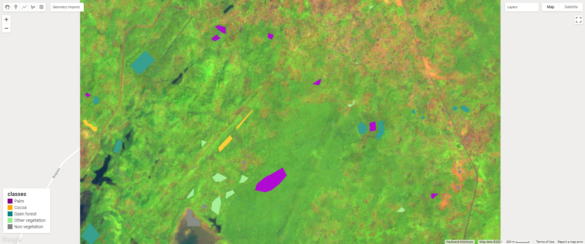
Step 1. Draw polygons for each land use class and save the polygons for each class as a separate geometry layer.
A few examples have been given in this tutorial. You can find them under ‘Geometry imports’ in the upper left of the map. Click on each layer to turn on/off the example layers. The national land use map of Ghana was used as reference for each strata.
Tips for drawing polygons: avoid ambiguous areas in which the land use isn’t clear; avoid edges (edge pixels in your imagery are likely to contain two different types of land use, which confuses the classifier.
Step 2: Merge the geometries of each class (each geometry contains training and validation areas for one strata) as one FeatureCollection.
// Step 2:  Merge the geometries of each class (each geometry contains training and validation areas for one strata) as one FeatureCollection.
var polygons = ee.FeatureCollection([
  ee.Feature(palm, {'class': 1}),
  ee.Feature(cocoa, {'class': 2}),
  ee.Feature(open_forest, {'class':3}),
  ee.Feature(other_veg, {'class': 4}),
  ee.Feature(non_veg, {'class': 5})
]);

// Set the names and colour for visulisation.
var class_name_list = ['Palm','Cocoa','Open forest','Other vegetation','Non vegetation']; // set class names
var colour_palette = ['purple','orange','teal','lightgreen','grey']; // set colour to each class
var class_number = ee.List(class_name_list).length().getInfo();

// View training and validation areas (different colours for each strata)
var fills = ee.Image().byte().paint({
  featureCollection: polygons,
  color: 'class',
});
Map.addLayer(fills, {palette: colour_palette,min:1, max: class_number}, 'Training and Validation polygons');
Step 3: Generate training and validation points within each strata using the sampleRegions function. Each pixel of the input feature image (at 10m scale in this example) that intersects with the training geometry (polygon) is converted to a Feature collection. Each output feature will have one property per band of the input image, as well as the ‘class‘ properties copied from the input feature. Note: In this example we are doing a cross validation…
var all_points = input_features
                  .sampleRegions({
                    collection: polygons,
                    properties: ['class'],
                    scale: 10,
                  //   tileScale: 8
                  })
                  .filter(ee.Filter.neq(
                      'B2', null)) // Remove null pixels.
                  .randomColumn() ; // add a ID column, which will be used to separate the points to training and validation dataset later.
7. Train a Random Forest model
Some technical details for those interested: Random Forest is an ‘ensemble classifier’, where a group of typically deep, Classification and Regression Tree (CART) classifier probabilities are averaged to predict the most likely class label of a pixel or object. Each tree within the ensemble employs random feature selection and bootstrap sampling with replacement for every split of the CART tree, followed by the averaging of probabilities across all trees, aims to mitigate against high variance. Take a look at some animations to explain this here.
Step 1: Randomly split the sample into training (70%) and validation dataset (30%).
You can uncomment the last line to view the selected training samples.
//Step 1: Randomly split the sample into training (70%) and validation dataset (30%)
var training = all_points.filter(ee.Filter.greaterThan('random',0.3));
var validation = all_points.filter(ee.Filter.lessThanOrEquals('random',0.3));
//print(training)
Step 2: Train a Random Forest classifier. You can tune the model by specifying the parameters (see the Google developers document here. In this example we are using 100 training trees.
//Step 2: train a Random Forest classifier
var trainedRf = ee.Classifier.smileRandomForest({numberOfTrees: 100}).train({
  features: training,
  classProperty:'class',
  inputProperties: bands_to_use // a list of selected band names
});
Step 3: Validate using an error matrix (note error matrix and confusion matrix are the same thing)
//Step 3: Validate using an error matrix
//Classify the validation data
var validatedRf = validation.classify(trainedRf);
Calculate the validation error matrix and accuracy for both classifiers by using the “errorMatrix” function to generate metrics on the re-substitution accuracy.
var validationAccuracyRf = validatedRf.errorMatrix('class', 'classification');
// Print validation accuracy results.
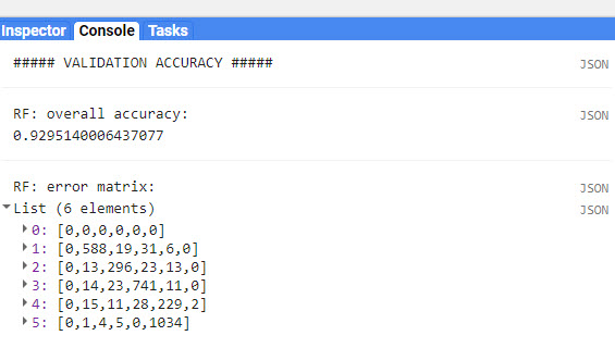
print('##### VALIDATION ACCURACY #####');
print('RF: overall accuracy: ', validationAccuracyRf.accuracy());
print('RF: error matrix: ', validationAccuracyRf);
From the error matrix we can see that the model has a lower accuracy for class 2 (cocoa). Cocoa is confused with Open Forest (class 3), Palm (class 1) and Other Vegetation.
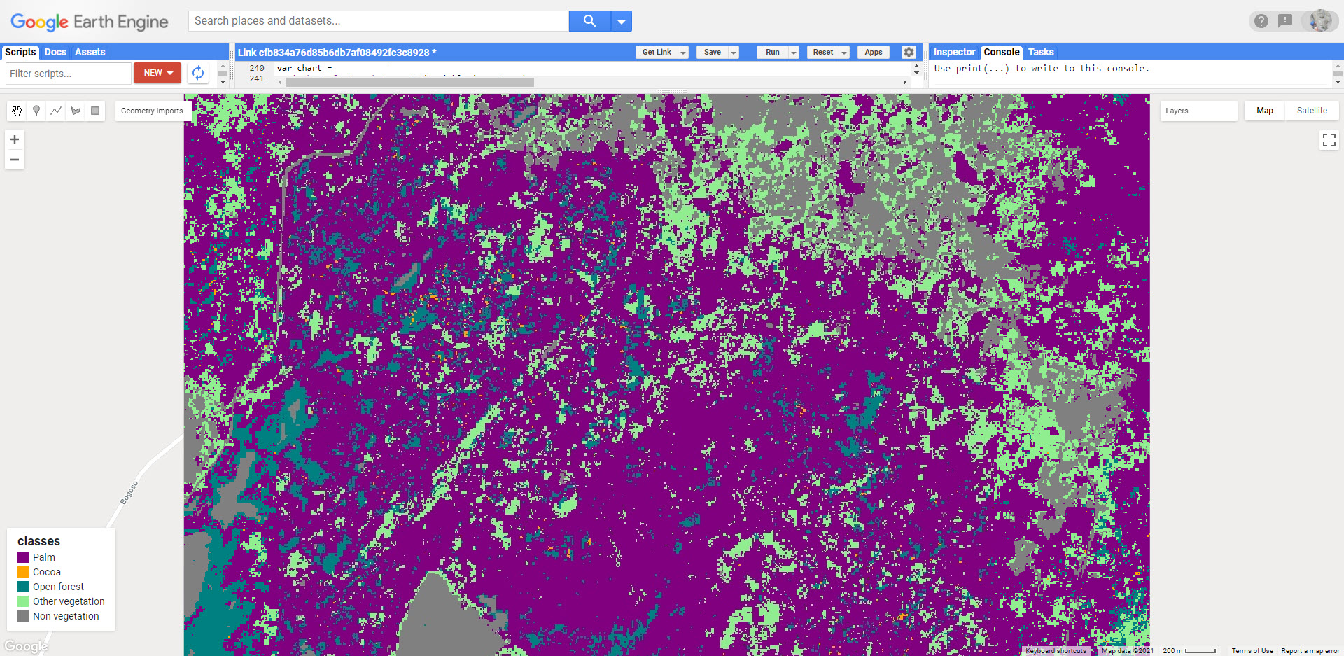
Step 4: Classify the image and add the map to viewer
//Step 4: Classify the image and add the map to the viewer
var classifiedRf = input_features.select(bands_to_use).classify(trainedRf);

var classVis = {min: 1, max: class_number, palette: colour_palette};
Map.addLayer(classifiedRf.clip(aoi), classVis, 'Classes (RF)');
img_process.addLegend('classes', colour_palette, class_name_list,class_number);
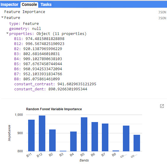
8. Feature importance
Feature importance is used to assess how useful each feature of the model input is in determining the output. This provides us an indication as to which pieces of information we should include in the model, and which ones we could leave out. Again, some technical details for those interested: The Random Forest classifier in Google Earth Engine is based on SMILE, where feature importance is calculated by summing up the decreases for each individual variable (GINI, information gain, etc.) over all trees in the forest. It is a fast way to calculate variable importance and is often very consistent with the permutation importance measure (more information refer to the GitHub page)
We use the classifer.explain() function in GEE to explore the variable importance of the trained Random Forest model.
var dict_featImportance = trainedRf.explain();
var variable_importance = ee.Feature(null, ee.Dictionary(dict_featImportance).get('importance'));
print('Variable Importance', variable_importance);

// Plot the variable importance as a bar chart
var chart =
  ui.Chart.feature.byProperty(variable_importance)
  .setChartType('ColumnChart')
  .setOptions({
  title: 'Random Forest Variable Importance',
  legend: {position: 'none'},
  hAxis: {title: 'Bands'},
  vAxis: {title: 'Importance'}
});
print(chart);
Discussion
Potential ways to improve classification accuracies:
- Compare the overall accuracy and confusion matrix between using texture information (Scenario 2) and not using it (Scenario 1)
- Will the accuracy further improve if we introduce other dataset?
- Explore texture information:
- kernel size
- Different RGB to greyscale transformation
- Improve the quality of the training dataset:
- import ground truth data from field work
- Using very high resolution satellite data with a matching date for sentinel-2 mosaics
- Will the accuracy further improve if we introduce other dataset?
- Sentinel-1 (Try this Analysis Ready data processing chain)
- Question: Using the knowledge you have gathered in this tutorial:
- What do you think can be used to improve the classification results?
- What is important when trying to achieve the most accurate classification?
- The classification accuracy for shaded cocoa remains the lowest among all classes.
- What data or method could improve the classification accuracy for shaded cocoa?

Responses