Lesson 1, Topic 1

In Progress

Copy of Incorporating EO into agricultural monitoring

nesrin s.

What do we want to know about a crop?

YouTube — Crop Monitoring: Biophysical Parameters – Introduction to biophysical parameters

Use of vegetation indices

Using remote sensing data, we can extract valuable information about the properties of vegetation. This allows us to measure the health of crops from general vegetation health to biophysical parameters such as chlorophyll content. Other biophysical parameters include the Leaf Area Index (LAI), leaf structure, dry matter content and many more. We can use vegetation indices (VI’s) to estimate these properties from remotely sensed imagery while correcting for disturbing effects of soil moisture, solar position, and other disturbances. VI’s should be calibrated to the study area and vegetation type with field measurements. Moreover, certain VI’s might not be the right choice for the type of vegetation you are studying.

Vegetation indices can be used in agriculture for the estimation of the following parameters:

Leaf Area Index (LAI) (from optical or radar imagery)
Vegetation cover (from optical or radar imagery)
Absorbed Photosynthetically Active Radiation (APAR) (from optical imagery)
Chlorophyll content (from optical imagery)
Canopy water content (from optical or radar imagery)
Biomass (from optical or radar imagery)
Carbon (from optical or radar imagery)
Structure of the canopy (from optical or radar imagery)

The site Index Database provides a list of indices that can be filtered by application, sensor, and both sensor and application.

Leaf Area Index (LAI)

The first parameter we will cover is the Leaf Area Index (LAI), which is the one-sided surface area of all leaves per unit of ground surface area. The value of LAI will depend on the crop you are interested in and the development stage of the plant. This can have an impact on the type of vegetation index which is best for estimating the LAI from satellite imagery.

The Normalized Difference Vegetation Index (NDVI) is a popular choice for assessing the health of vegetation. It uses the Near infra-red (NIR) and red reflectance in its formula. The value range is between -1.0 to 1.0 with negative values corresponding to water, snow, rocks, and bare soil, low positive values corresponding to sparse vegetation, and high positive values to dense vegetation.

NDVI = frac{NIR-RED}{NIR+RED}

The saturation of NDVI is seen in vegetation with LAI values over 4-5. Source: (Clevers et al., n.d.)

An issue with using NDVI to estimate LAI becomes apparent at higher LAI values where the index becomes saturated. This can be in dense tropical forests or in other crops with large amounts of leaves. Other vegetation indices might be preferred based on your application, such as ratio vegetation indices which are more sensitive compared to NDVI (Towers et al., 2019).

Remote Sensing for LAI estimation

This next video explains the process of LAI estimation using the WDVI (weighted difference vegetation index) though this process can be expanded to other statistical vegetation indices.

Other than the WDVI and NDVI there are many more vegetation indices which can be used for estimating LAI. The site L3 Harris Geospatial contains a brief overview of these indices which are present in their software ENVI.

Chlorophyll estimation from RS imagery

Chlorophyll is another crop property which can be measured remotely to assess plant health. In the following video, we will explain how to calculate the chlorophyll content at the leaf and at canopy level. Jan Clevers illustrates two vegetation indices, the CVI (Chlorophyll vegetation index) and CI_green (Green Chlorophyll index), the equations of which you can find below.

CVI equation

CVI = frac{NIR}{GREEN}*frac{RED}{GREEN}

CI_green equation

CVI = frac{NIR}{GREEN}*frac{RED}{GREEN} - 1

Chlorophyll monitoring using remote sensing

Crop modeling

Models serve to answer specific questions in many different areas, such as economy, environmental sciences, hydrology, and agronomy. They are a simplified version of reality which is constituted by assumptions and a way to represent relevant processes. The two overarching model types are statistical or empirical models and mechanistic or process-based models. The former work with the statistical relationship between variables and set up based on observed values. The latter rely more heavily on assumptions about the processes involved and describe them with mathematical equations. The main characteristics of these model types are:

Statistical/empirical models :

Rely on observed values
Establish a direct statistical relationship between inputs and outputs, e.g., through regression modeling
Advantages: Simple to set up
Disadvantages: Require ground truth data and usually do not perform well for settings other than the ones they were designed for

Mechanistic/process-based models:

Use a basic understanding of biophysical system processes and causality
Advantages: Explanatory capacity, use without ground truth data is possible, as well as extrapolation into unknown settings
Disadvantages: Require system understanding and rely on relevant assumptions, which may not hold true (increases uncertainty)

(Weiss et al., 2020)

Crop models are often a combination of these two model types. Which model type is suited for a given agricultural application depends on the application and the circumstances. The same characteristic may also be modeled both by statistical and mechanistic approaches. For example, crop yield can be modeled either by simply relating it to one or several of the above-mentioned vegetation indices from remote sensing data or by integrating these indices into an existing mechanistic model. Another example is to combine a crop’s growing cycle with thermal time, the time of growing days of a crop in relation to the temperature, inferred from remote sensing data.

Crop models are valuable tools that can help predict an outcome in a specific genetic, environmental, or management setting (scenario testing) and thus help generate information that is otherwise unavailable, expensive, or cumbersome to obtain. Integrated with ground-based data, crop growth and yield forecasting can be connected to decision-support systems that help stakeholders make informed decisions about the food system (learn about the European Union’s MARS yield forecasting system and why it is important here).

Sensor selection

Which sensor characteristics for which task?

How remote sensing data can serve agricultural monitoring depends on its characteristics and the task to fulfil. See below three example time series of different remotely sensed imagery.

MODIS imagery (left) is provided daily, Landsat imagery (middle) every 16 days and Sentinel-2 imagery (right) every 5 days.

To determine the right sensor for the job, it is crucial to think about the following questions:

Which domain? [Sensor type]

Optical imagery allows to calculate a range of indices relevant to agriculture and is widely applied in agriculture and operational monitoring systems (Migdall et al., 2018). However, radar imagery can penetrate clouds and allows image acquisition at day and night times, which enables reliable observations and can be used for crop classification, crop monitoring, and soil and vegetation moisture monitoring. (Steele-Dunne et al., 2017).

How detailed? [Spatial resolution]

Mixed pixels are ambiguous and complicated to unmix due to:

Potential temporal shifts between winter and summer crops
Adjacent crops change with rotations

The spatial resolution needs to be fine enough to have a crop-specific signal, but not too coarse to limit unnecessary noise and excessive computations. Spatial requirements will vary according to landscape complexity (e.g., Duveiller & Defourny, 2010).

Imagery and derived crop-specific masks for six agricultural sites. The imagery is displayed using the NIR band in the red channel, the Red band in the green, and the SWIR band in the blue. (Source: Duveiller & Defourny(2010)).

What geographic extent? [Swath]

Are we looking at localized precision agriculture?

(a) Airborne hyperspectral imagery acquired with a VNIR sensor on board a UAV yielding 40-cm resolution. (b) Resampled to 50-m pixels to assess the aggregation effects on fluorescence retrieval. (c)–(g) Complexity of planting grids/orientations. Images are shown in color composites using green, red, and NIR bands. (Source: Zarco-Tejada et al. 2013)

…or at global/regional agricultural monitoring?

Probability of deficit (P N 0.3) and progress of the season as of 1 November 2009. (Source: Meroni et al.(2014)).

What temporal coverage? [Archive length]

Many applications require comparing with past events to characterize similar years, anomalies, and trends. Then, we need the longest possible archives.

Examples of yield regression models and their respective fAPAR time series for winter cereal production across Europe. (Source: López-Lozano et al. (2015))

Which sensor type to use [Data selection]

So, how to combine the different considerations to select one or more sensors that serve the intended purpose?

To evaluate multiple dimensions, we can resume them into a spider plot:

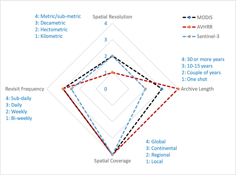
Comparison of remote sensing instrument characteristics

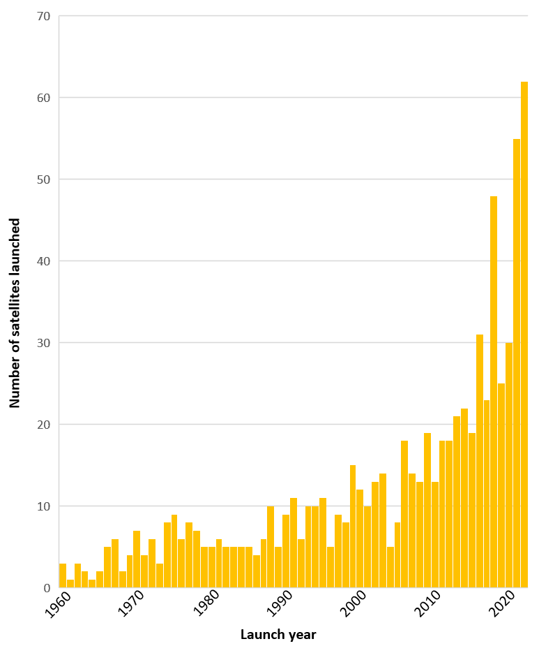
As you can see in the chart, the number of meteorological and Earth observation satellites launched is rapidly increasing and so are the observation capacity and spatial resolution. The launch of Sentinel-2A and Sentinel-2B provides a 5-day revisit time, and in combination with Landsat 8 and 9, this increases even more. Solutions like the Google Earth Engine (GEE) allow for managing such heavy loads of data. So, is coarse spatial resolution obsolete? The answer is “no”.

A possible strategy is to wait for comprehensive archives to be constituted from the more recently launched high spatial resolution sensors. Alternatively, imagery from different sensors can be combined in various ways to benefit from their respective characteristics, as shown below. Fine spatial resolution and more recent imagery like Sentinel-2 can be used synergistically with long-standing image archives like Landsat. A combination of sensors can also help to fill image gaps due to cloud cover or create denser time series with more frequent observations. These time series can then be integrated into crop models.

Explore the interactive charts below!

(Duveiller, 2015)

Another example of synergistic sensor use is to combine different radar frequencies. Each frequency responds to a different plant characteristic, and their combination can help distinguish crops and monitor their growth stages.

Integration of Data from RADARSAT-2, ALOS, and TerraSAR-X, Manitoba (Canada). Source: McNairn et al. (2021).

How to apply EO data for agricultural monitoring?

Incorporating EO data for agricultural monitoring requires you to know which crop parameter(s) you want to look at, where, and under which circumstances. Vegetation indices like the optical-based LAI can be related to information that is essential for food security, such as yield. The success of interventions like fertilizer application or irrigation measures is therefore often measured by monitoring LAI.

But not every vegetation index can be derived from every sensor at the required level of detail. It is key to consider the sensor type needed for the job, the spatial resolution, geographic extent, and archive length to identify appropriate sensors for the task. For some applications, it can be useful to combine multiple sensor systems from the same domain, e.g., to extend the image archive, or to combine data from different domains, e.g., optical and radar imagery, to close data gaps due to cloud cover.

Once the appropriate remote sensing data is identified, it can be used to characterize the agricultural landscape and determine crop type and phenology. Integrated into a crop model, remote sensing data can support management decisions by simulating the impact of climate change on crop growth, of specific irrigation practices on yield, or by forecasting crop performance regarding national or regional food security.

In summary, successful agricultural monitoring with EO technology necessitates selecting a good parameter for what we want to observe, the right respective sensor or set of sensors for the task, and an approach to the application that yields relevant outputs.

Credit

This topic was created with the help of learning materials that were kindly provided by:

– EO College: Land in Focus – Basics of Remote Sensing, Land in Focus – Agriculture & Food
– NASA Applied Remote Sensing Training Program (ARSET): McNairn, H.; Dingle-Robertson, L.; Fitrzyk, M.; Ramoino, F.; Karadimou, G.; Roth, T.; Bontemps, S.; Defourny, P. (2021). Agricultural Crop Classification with Synthetic Aperture Radar and Optical Remote Sensing. NASA Applied Remote Sensing Training Program (ARSET).
– The European Space Agency (ESA): 6th ESA Advanced Training Course on Land Remote Sensing 2015 and from the 9th Advanced Training Course on Land Remote Sensing with the focus on Agriculture 2019

Sources and further readings

Sources

Clevers, J. G. P. W., Lammert, K., & Brede, B. (n.d.). Land in Focus – Agriculture & Food. Crop Monitoring: Biophysical Parameters. EO College. https://eo-college.org/courses/agriculture-and-food/lessons/crop-monitoring-biophysical-parameters/

Duveiller, G. (2015, September 17). Agriculture Monitoring. 6th ESA Advanced Training Course on Land Remote Sensing, Bucharest. https://eo4society.esa.int/wp-content/uploads/2021/02/D4T1b_LTC2015_Duveiller.pdf

Duveiller, G., & Defourny, P. (2010). A conceptual framework to define the spatial resolution requirements for agricultural monitoring using remote sensing. Remote Sensing of Environment, 114(11), 2637–2650. https://doi.org/10.1016/j.rse.2010.06.001

Henrich, V. H., Krauss, G. K., Götze, C. G., & Sandow, C. S. (2012). IDB – Index DataBase. Index Database. https://www.indexdatabase.de/

Food and Agriculture Organization of the United Nations (FAO) (2015). Yield gap analysis of field crops: Methods and case studies. https://www.fao.org/3/i4695e/i4695e.pdf

L3 Harris Geospatial. (2020). Broadband Greenness. https://www.l3harrisgeospatial.com/docs/broadbandgreenness.html

Lobell, D. B., & Burke, M. B. (2010). On the use of statistical models to predict crop yield responses to climate change. Agricultural and Forest Meteorology, 150(11), 1443–1452. https://doi.org/10.1016/j.agrformet.2010.07.008

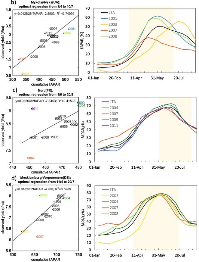
López-Lozano, R., Duveiller, G., Seguini, L., Meroni, M., García-Condado, S., Hooker, J., Leo, O., & Baruth, B. (2015). Towards regional grain yield forecasting with 1km-resolution EO biophysical products: Strengths and limitations at pan-European level. Agricultural and Forest Meteorology, 206, 12–32. https://doi.org/10.1016/j.agrformet.2015.02.021

McNairn, H., Dingle-Robertson, L., Fitrzyk, M., Ramoino, F., Karadimou, G., Roth, T., Bontemps, S., & Defourny, P. (2021). Agricultural Crop Classification with Synthetic Aperture Radar and Optical Remote Sensing. NASA Applied Remote Sensing Training Program (ARSET). https://appliedsciences.nasa.gov/join-mission/training/english/arset-agricultural-crop-classification-synthetic-aperture-radar-and

Mason-D’Croz, D., Sulser, T. B., Wiebe, K., Rosegrant, M. W., Lowder, S. K., Nin-Pratt, A., Willenbockel, D., Robinson, S., Zhu, T., Cenacchi, N., Dunston, S., & Robertson, R. D. (2019). Agricultural investments and hunger in Africa modeling potential contributions to SDG2 – Zero Hunger. World Development, 116, 38–53. https://doi.org/10.1016/j.worlddev.2018.12.006

Meroni, M., Fasbender, D., Kayitakire, F., Pini, G., Rembold, F., Urbano, F., & Verstraete, M. M. (2014). Early detection of biomass production deficit hot-spots in semi-arid environment using FAPAR time series and a probabilistic approach. Remote Sensing of Environment, 142, 57–68. https://doi.org/10.1016/j.rse.2013.11.012

Migdall, S., Brüggemann, L., & Bach, H. (2018). Earth Observation in Agriculture. In C. Brünner, G. Königsberger, H. Mayer, & A. Rinner (Eds.), Satellite-Based Earth Observation (pp. 85–93). Springer International Publishing. https://doi.org/10.1007/978-3-319-74805-4_9

OSCAR. (n.d.). List of all satellites. Observing Systems Capability Analysis and Review Tool (OSCAR). https://space.oscar.wmo.int/satellites

Pasquel, D., Roux, S., Richetti, J., Cammarano, D., Tisseyre, B., & Taylor, J. A. (2022). A review of methods to evaluate crop model performance at multiple and changing spatial scales. Precision Agriculture, 23(4), 1489–1513. https://doi.org/10.1007/s11119-022-09885-4

Steele-Dunne, S. C., McNairn, H., Monsivais-Huertero, A., Judge, J., Liu, P.-W., & Papathanassiou, K. (2017). Radar Remote Sensing of Agricultural Canopies: A Review. IEEE Journal of Selected Topics in Applied Earth Observations and Remote Sensing, 10(5), 2249–2273. https://doi.org/10.1109/JSTARS.2016.2639043

Towers, P. C., Strever, A., & Poblete-Echeverría, C. (2019). Comparison of Vegetation Indices for Leaf Area Index Estimation in Vertical Shoot Positioned Vine Canopies with and without Grenbiule Hail-Protection Netting. Remote Sensing, 11(9), 1073. https://doi.org/10.3390/rs11091073Weiss, M., Jacob, F., & Duveiller, G. (2020). Remote sensing for agricultural applications: A meta-review. Remote Sensing of Environment, 236, 111402. https://doi.org/10.1016/j.rse.2019.111402

van Ittersum, M. K., & Rabbinge, R. (1997). Concepts in production ecology for analysis and quantification of agricultural input-output combinations. Field Crops Research, 52(3), 197–208. https://doi.org/10.1016/S0378-4290(97)00037-3

Weiss, M., Jacob, F., & Duveiller, G. (2020). Remote sensing for agricultural applications: A meta-review. Remote Sensing of Environment, 236, 111402. https://doi.org/10.1016/j.rse.2019.111402

Zarco-Tejada, P. J., Suarez, L., & Gonzalez-Dugo, V. (2013). Spatial Resolution Effects on Chlorophyll Fluorescence Retrieval in a Heterogeneous Canopy Using Hyperspectral Imagery and Radiative Transfer Simulation. IEEE Geoscience and Remote Sensing Letters, 10(4), 937–941. https://doi.org/10.1109/LGRS.2013.2252877

Discussion

Visit discussion for more topics

Agriculture & Livestock

Incorporating EO into agricultural monitoring

Posted by EO College on December 16, 2022 at 10:35 am

EO College replied 1 year, 7 months ago 1 Member · 0 Replies
0 Replies

Sorry, there were no replies found.