L1T1 – Fundamentals of Remote Sensing
A history detour
Did you know? The term ‘remote sensing’ actually arose from an unpublished paper in the early 1960s by the staff of the Naval Research Geography Branch. Before this, different terms to describe the procedures used in earth observation.
If you want to explore the historical milestones that led us to remote sensing as we know it today, take your time to scroll through the timeline animation below. Many of the terms that are mentioned in the interactive time bar will come up during a later stage of this course and will also be essential knowledge to put into practice in our practical courses that will follow after this course.
While most theories that apply to remote sensing instruments were formulated long before they were transformed into physically meaningful technologies, they are still valid today: from the drive of creating knowledge and over-achieving military advances to using remote sensing for good causes and to solve the world’s greatest environmental problems.
Remote sensing (RS) includes techniques and methods to observe the Earth’s surface, usually by the formation of an image in a position − stationary or mobile − at a distance remote from that surface (after Buiten & Clevers, 1993). In remote sensing, electromagnetic (EM) radiation coming from an object is being measured. The two phases (measurement phase: a-d and second phase: e-g) are explained in the explorable explanation below.
L1T2 – Electromagnetic waves and their spectrum
c = \lambda f
L1T3 – Electromagnetic waves and their spectrum
L1T4 – Reflection and Absorption
L2T1 – Passive Imaging Techniques
List of passive instruments
Below you can find two explorable animations that present a selection of the most important remote sensing sensors that can be found in the passive remote sensing domain.
Optical sensors
Radar sensors
L2T2 – Active Imaging Techniques
Radar bands
Microwave frequencies are labelled in Bands. Perhaps you stumbled on this seemingly confusing nomenclature of X-Band, C-Band or L-Band when dealing with radar images. Learn what these labels mean and how to remember the bands.
Field scenario
City scenario
Snow scenario
L3T1 – Spatial Resolution
Comparison of spatial resolutions
In the interactive element below, you can slide through the variations of (mostly) commonly used sensors. They visualize a part of the Skukuza rest camp, which is located in the Kruger National Park, South Africa. Explore how details get mixed or disappear completely.
In recent years, more high-resolution data became freely available and this trend will prevail in the upcoming decades. While low-resolution (coarse) data sets have dominated the past, high-resolution (fine) data will be the go-to input information for state-of-the-art remote sensing science, also taking into account the steadily improving processing possibilities on personal computers and cloud servers.
Mixed pixel problem
Mixed pixels represent a classic problem in remote sensing applications as there existent heavily depends on the pixel resolution we are looking at. With lower spatial resolution (smaller pixel size), reflections from more surrounding objects are combined into one resolution cell. Hence, the original cell we are looking at will exhibit image statistics from a variety of neighboring pixels. Have a look at the image slider below and see how lowering the spatial resolution leads to mixed pixels containing less deta. Note how some of the small buildings get mixed up with the surrounding trees in the 30 m imagery.
If objects are larger than, or at least equal to, the spatial resolution of the respective sensor, they will be mapped in our data sets. There is also the chance that the brightness of an object smaller than the cell size (e.g. a building) is high enough to impact the cell statistics. If this is the case, analysis could be carried out on a sub-pixel domain to enable the identification of parts of a resolution cell.
L3T2 – Temporal Resolution
L3T3 – Spectral Resolution
L3T4 – Radiometric Resolution
What is radiometric resolution?
The radiometric domain is also referred to as ‘color depth’ and is defined as the sensitivity to the magnitude of the EM energy. Thus, it characterizes how finely a given sensor can receive and divide the radiance between the different bands. Explore the animation on the right to investigate the difference between lower and higher radiometric at comparable spatial resolution. A greater resolution increases the range of intensities that a sensor can distinguish.
Source: ESA 2009
L4T1 – Preprocessing – Optical
Value conversion
The conversion from DN to radiance and reflectance is an important step in the preprocessing. In the case of Sentinel-2 and Landsat data, we are usually interested in the bottom-of-atmosphere (BOA) reflectance, which is, in contrast to the top-of-atmosphere (TOA) reflectance, corrected for atmospheric impacts and can thus directly be interpreted. However, the initially available data sets are being converted from DN to TOA format. For the conversion, the data is rescaled using sensor specific equations containing information about sun-related angles and other parameters. As an example fur such a conversion, the expression used to correct Landsat 8 OLI data is given below.
\rho\lambda = \frac{M_{\rho}Q_{cal} + A_{\rho}}{\cos \theta_{SZ}}ρλ = TOA reflectance
Mρ = multiplicative rescaling factor
Qcal = DN (quantized & calibrated)
Aρ = additive rescaling factor
θSZ = local solar zenith angle, θSZ = 90° – θSE = local sun elevation angle
Using these equations, we can compute TOA data which is not subject to strong illumination geometry difference-related effects.
Other preprocessing steps
Below you can explore a couple of additional algorithms and how they influence the remote sensing image visually (and statistically).
Stretching of grey level values to allow better visibility and pixel distinction
Geometric correction to remove spatial distortions
High pass filter to sharpen edges and increasing contrast
Low pass filter to smoothen satellite imagery
L4T2 – Preprocessing – SAR
L4T3 – Sensor accurracy
Accuracy and precision
In everyday language, accuracy and precision both relate to quality and may be used as synonyms. In remote sensing (and other scientific disciplines), they have specific meanings:
Accuracy refers to the distance of a measurement (or prediction) to the true value. It can also be referred to as trueness. An accurate measurement produces results that are close to the true value.
Precision refers to the repeatability or reproducibility of a measurement. It refers to the spread that occurs if the measurement (or prediction) is repeated under the same conditions. A precise measurement produces results that are close to each other, no matter their distance from the true value.
Root Mean Square Error (RMSE)
The RMSE is a measure for the accuracy of a RS product, i.e. the distance of RS predictions from the corresponding ground truth measurements. It is defined as:
RMSE=\sqrt{\frac {\sum(\hat{x}_i - x_i)^2} n}It should be used when comparing metrics that should by definition be same quantities. For example, if Leaf Area Index ( LAI in m2/m2) is derived from RS data it can be compared to ground truth LAI data with the RMSE. The RMSE has the same physical unit as the RS product and the ground truth. It should be noted that the RMSE weights large errors heavier than smaller errors because of the square. Also, positive (overestimation) and negative (underestimation) errors have the same impact on RMSE.
Tutorial
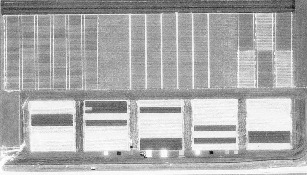
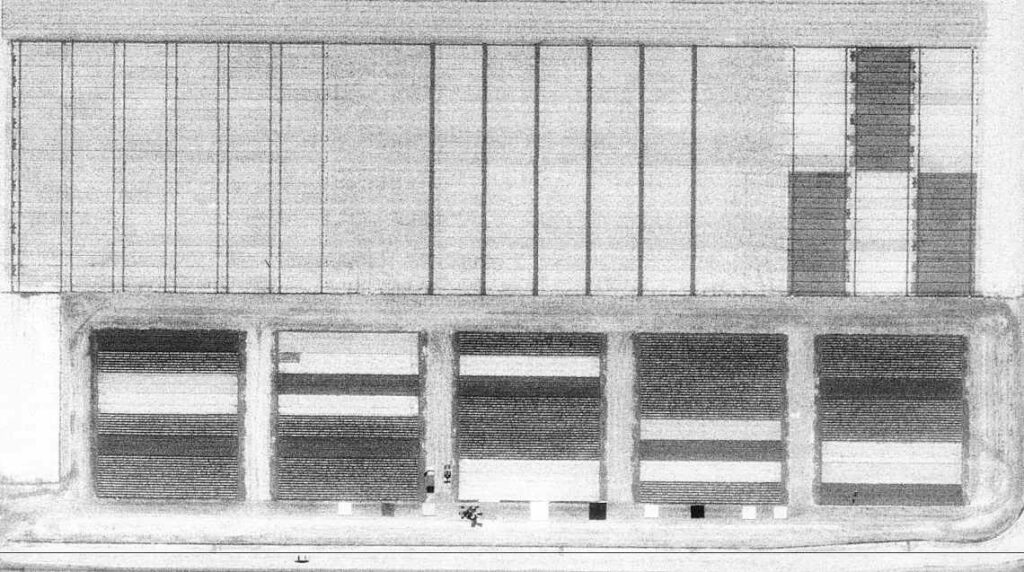
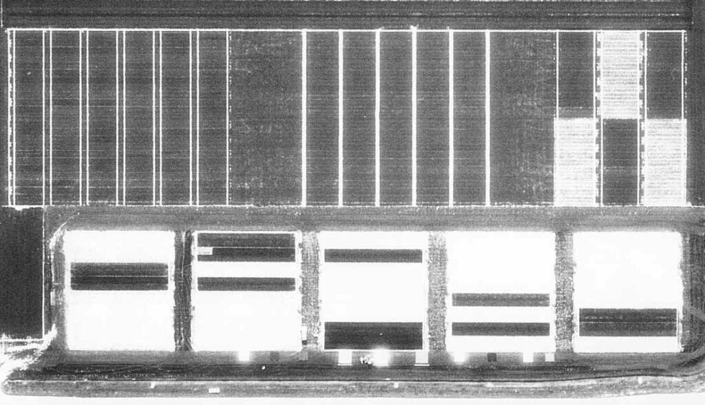
The remainder of this topic is a practical exercise where you will first derive reflectance’s from aerial images then validate your calibration by comparing the derived values to ground truth data. This tutorial is run in two parts, first you will evaluate the digital pixel values (DN) in three black-and-white images corresponding to green, red and near infrared bands shown below.
L5T1 – Visual Image Interpretation
L5T2 – Classification
The following presentation summarizes the main points of the knowledge clip above. You can use it to review what you’ve just learned.
The presentation below reviews some main topics and the classification algorithms discussed.
The following book reviews the main concepts of the knowledge clip. You can use it to supplement your learning.
L5T3 – Classification Accuracy Assessment
Overall accuracy and overall error
Overall accuracy (OA) tells us the proportion of validation sites that were classified correctly. The diagonal of the matrix contains the correctly classified sites. To calculate the overall accuracy you sum up the number of correctly classified sites and divide it by the total number of reference sites.
{Overall\, Accuracy} = \frac {(25 +32+26)} {106} = 0.79Overall error represents the proportion of validation sites that were classified incorrectly. This is thus the complement of the overall accuracy (accuracy + error = 100%). So you can calculate the overall error from the overall accuracy, or you add the number of incorrectly classified sites and divide it by the total number of reference sites.
{Overall\, Error} = 1 - {Overall\, Accuracy} = 1-0.78 =0.22{Overall\, Error} = \frac{(7+6+5+3+0+2)}{106} = 0.22In our example the overall accuracy is 78% and the overall error is 22%.
Producer’s accuracy
Producer’s accuracy (PA), also known as sensitivity (in statistics) and recall (in machine learning), is a measure for how often real features on the ground are correctly shown on the classified map. So it is the map accuracy from the point of view of the map maker (producer). It is calculated per class by dividing the number of correctly classified reference sites by the total number of reference sites for that class (= column totals).
PA\, water = \frac{25}{38} = 0.66User’s accuracy
User’s accuracy (UA), also known (in statistics and machine learning) as precision, is a measure for how often the class on the map will actually be present on the ground. So it is the map accuracy from the point of view of the map user. It is calculated per class by dividing the number of correct classifications by the total number of classified sites for that class (= row totals).
UA\, water = \frac{25}{30} = 0.83Error of omission
The error of omission is the proportion of reference sites that were left out (or omitted) from the correct class in the classified map. This is also sometimes referred to as a Type II error or false negative rate. The omission error is complementary to the producer’s accuracy, but can also be calculated for each class by dividing the incorrectly classified reference sites by the total number of reference sites for that class.
Omission\,error\,water = \frac{7+6}{38} = 0.34 \\OR\\ 1-PA\,water = 1-0.66=0.34Error of commission
The error of commission is the proportion of classified sites that were assigned (or committed) to the incorrect class in the classified map. This is also sometimes referred to as a Type I error or false discovery rate. The commission error is complementary to the user’s accuracy, but can also be calculated for each class by dividing the incorrectly classified sites by the total number of classified sites for that class.
Commission\,error\,water = \frac{5+0}{30} = 0.17 \\OR\\ 1-UA\,water = 1-0.83=0.17L5T4 – Image Classification Tutorial
L5T5 – Image Classification Tutorial
L5T6 – Time Series Analysis
\frac{NIR-RED}{NIR+RED}