
Accuracy assessment of remote sensing products
Calibration and validation are key to creating suitable remote sensing-based products and providing information on their quality and reliability. EO products should be assessed quantitatively for:
- Model or method verification: This can be based on a calibration dataset only, to evaluate the performance of a classification model or an inversion algorithm to support model parameterization, model calibration, or serve as a quality control procedure.
- Model, method, or product benchmarking: This is based on reference data targeting disagreement areas to compare the performance of different processing methods/products to support the selection of a model or a method.
- EO product map accuracy assessment (validation): This is based on a validation dataset to quantify the accuracy of the information based on a statistically-sound strategy to support the decision to be made from this EO product.
Decisions based on maps with unknown accuracy might lead to serious surprises!
The Committee on Earth Observations (CEOS) categorizes product validation into the following four stages:
In an accuracy assessment, a map is compared with validation data. Based on the sampling protocol for the collected validation data, a confusion or error matrix can be constructed. This confusion matrix is a cross-tabulation of the class labels allocated by map and validation data. Usually, the map classes are represented in rows and the reference classes in columns.
The confusion matrix allows for the calculation of the following accuracy metrics (Congalton, 1991):
- Overall accuracy & Overall error
- Producer’s accuracy
- User’s accuracy
- Errors of omission
- Errors of commission
The table below gives an example of a confusion matrix for classification with 3 classes (water, grassland, and cropland). We will use this matrix to illustrate how to calculate the various accuracy metrics.
| Classified/ Reference | Water | Grassland | Cropland | Total |
| Installation | 25 | 5 | 0 | 30 |
| Grassland | 7 | 32 | 2 | 41 |
| Cropland | 6 | 3 | 26 | 35 |
| Total | 38 | 40 | 28 | 106 |
* Note that this calculation is valid for validation data collected using random sampling, i.e., if sample inclusion probability is the same for each validation location. In case of unequal inclusion probability, i.e., an equal number of sample sites selected regardless of the stratum area in stratified sampling, different accuracy estimation formulas are used. Accordingly, confidence intervals for the accuracy metrics are calculated differently, but this is outside the scope of this module. Section 4.2 in Olofsson et al. (2014) includes good practice recommendations when assessing map accuracy.
Classification accuracy assessment
Explore below different accuracy and error measures
Overall accuracy and overall error
Overall accuracy (OA) tells us the proportion of validation sites that were classified correctly. The diagonal of the matrix contains the correctly classified sites. To calculate the overall accuracy you sum up the number of correctly classified sites and divide it by the total number of reference sites.
OA = frac{25 + 32 + 26}{106} = 0.79Overall error represents the proportion of validation sites that were classified incorrectly. This is thus the complement of the overall accuracy (accuracy + error = 100%). So you can calculate the overall error from the overall accuracy, or you add the number of incorrectly classified sites and divide it by the total number of reference sites.
OE = 1 - OA = 1 - 0.78 = 0.22
OE = frac{7 + 6 + 5 + 3 + 0 + 2}{106} = 0.22In our example, the overall accuracy is 78% and the overall error is 22%.
Producer’s accuracy
Producer’s accuracy (PA), also known as sensitivity (in statistics) and recall (in machine learning), is a measure of how often real features on the ground are correctly shown on the classified map. So it is the map accuracy from the point of view of the mapmaker (producer). It is calculated per class by dividing the number of correctly classified reference sites by the total number of reference sites for that class (= column totals).
PA_{water} = frac{25}{38} = 0.66User’s accuracy
User’s accuracy (UA), also known (in statistics and machine learning) as precision, is a measure of how often the class on the map will actually be present on the ground. So it is the map accuracy from the point of view of the map user. It is calculated per class by dividing the number of correct classifications by the total number of classified sites for that class (= row totals).
UA_{water} = frac{25}{30} = 0.83Error of omission
The error of omission is the proportion of reference sites that were left out (or omitted) from the correct class in the classified map. This is also sometimes referred to as a Type II error or false negative rate. The omission error is complementary to the producer’s accuracy, but can also be calculated for each class by dividing the incorrectly classified reference sites by the total number of reference sites for that class.
OME_{water} = frac{7+6}{38} = 0.34OR
1 - PA_{water} = 1 - 0.66 = 0.34Error of commission
The error of commission is the proportion of classified sites that were assigned (or committed) to the incorrect class in the classified map. This is also sometimes referred to as a Type I error or false discovery rate. The commission error is complementary to the user’s accuracy, but can also be calculated for each class by dividing the incorrectly classified sites by the total number of classified sites for that class.
COE_{water} = frac{5 + 0}{30} = 0.17OR
1 - UA_{water} = 1 - 0.83 = 0.17In-situ data collection
In-situ data for EO in agriculture
In-situ data for EO in agriculture can be crop type data, phenology, agricultural practices, biophysical variables (e.g., LAI, LAIeff, FAPAR or FCOVER, soil moisture, yield, crop height, density,…), or other data collected on the ground or obtained from data analysis (e.g. photo-interpretation) (ESA Land Training).
In-situ data collection: two different objectives
Objective 1: In-situ data is used for calibration (training): sampling to cover the diversity of situations existing in the study site (possibly the national territory) to represent the range of possible signatures for the different elements of interest (i.e. croplands vs non-croplands on one hand and, the five main crop types and the other frequent crops on the other hand).
Objective 2: In situ data for validation to estimate the accuracy of the product (with a confidence interval) using a statistically-sound sampling to be objective and independent; for logistic reasons, sampling is not strictly random but 2-stage sampling (e.g., with few randomly-sampled primary sampling units and elementary sampling units sampled with a cost-efficient, not strictly random sampling scheme) to assess the crop types.
Calibration and validation field campaigns for cropland and crop type can be all combined, but the sampling design should be explicitly different to be independent. In agricultural mapping, sometimes two field campaigns are needed for early and end-of-season maps when all crop types cannot be identified during the mid-season campaign.
Requirements for in-situ samples
Gathering in-situ data, for example, to validate a crop classification map, is not a trivial task. The sampling design should fulfill the following criteria (Stehman & Foody, 2019):
- Satisfy the conditions defining a probability sampling design
- Easy to implement for both selecting the sample and producing estimates for accuracy
- Cost-effectiveness
- Readily allows for increasing or decreasing the sample size
- Precise in the sense that estimates have small standard errors
- Unbiased estimator of variance
- Spatially well-distributed samples across the study area
A typical approach can be conducted in the following three steps:
Stratification
Stratification according to existing agroecological zoning to sample the range of diversity.

On-screen visual interpretation
On-screen visual interpretation to select samples (min. 1 ha) of land cover types different than cropland on recent aerial photographs, Google Earth, or Bing imagery to capture the diversity of non-cropland land cover types. The sample distribution between strata could also consider the stratum size and their respective diversity.

Ground survey
Ground survey to delineate crop type samples (min. 1 ha, but larger is better): For each stratum. No strict sampling design but need to capture each crop’s diversity. Visual delineation could use the most recent color composite.

Innovative methods to gather in-situ data
Challenges to data collection
While a sampling design may be straightforward for a smaller study area in a controlled environment, a larger study site size, inaccessibility of parts of the area, and temporal variability (crop phenology, management practices), can complicate things. Thus, challenges for in-situ data collection are:
- To capture the entire diversity of the agriculture patterns
- To cover the full diversity of the crop types of interest and all the minor crop types (it is important to define the targeted crop types to emphasize the field data collection on them and to capture all the gradients in crop growing conditions of the crop types of interest)
- To integrate the quality of the in-situ data (labeling error, location error, editing error, etc.) as the in-data quality is of paramount importance
- To ensure the spatial distribution of the in-situ data across the whole study area to avoid local overfitting of the classification model to specific growing conditions
- To use spatially independent in situ data for robust accuracy assessment (the closer the calibration and validation data set are in space, the more the accuracy metrics represent the quality of the classification model rather than the quality of the entire map)
Novel ways of data collection
Where, from a statistical point of view, traditional sampling with random or stratified sampling schemes may be the most adequate ones to fulfill the above-mentioned criteria, conventional ways to sample ground data often lack the scale that is needed for modern applications. Therefore, novel ways to survey agriculture in a resource-efficient manner are increasingly explored. These include new ways of conducting surveys, using administration data, as well as crowdsourcing, for example through social networks, and farmers‘ data from farm management tools. Find some examples of each of these in-situ data types below.
The windshield survey
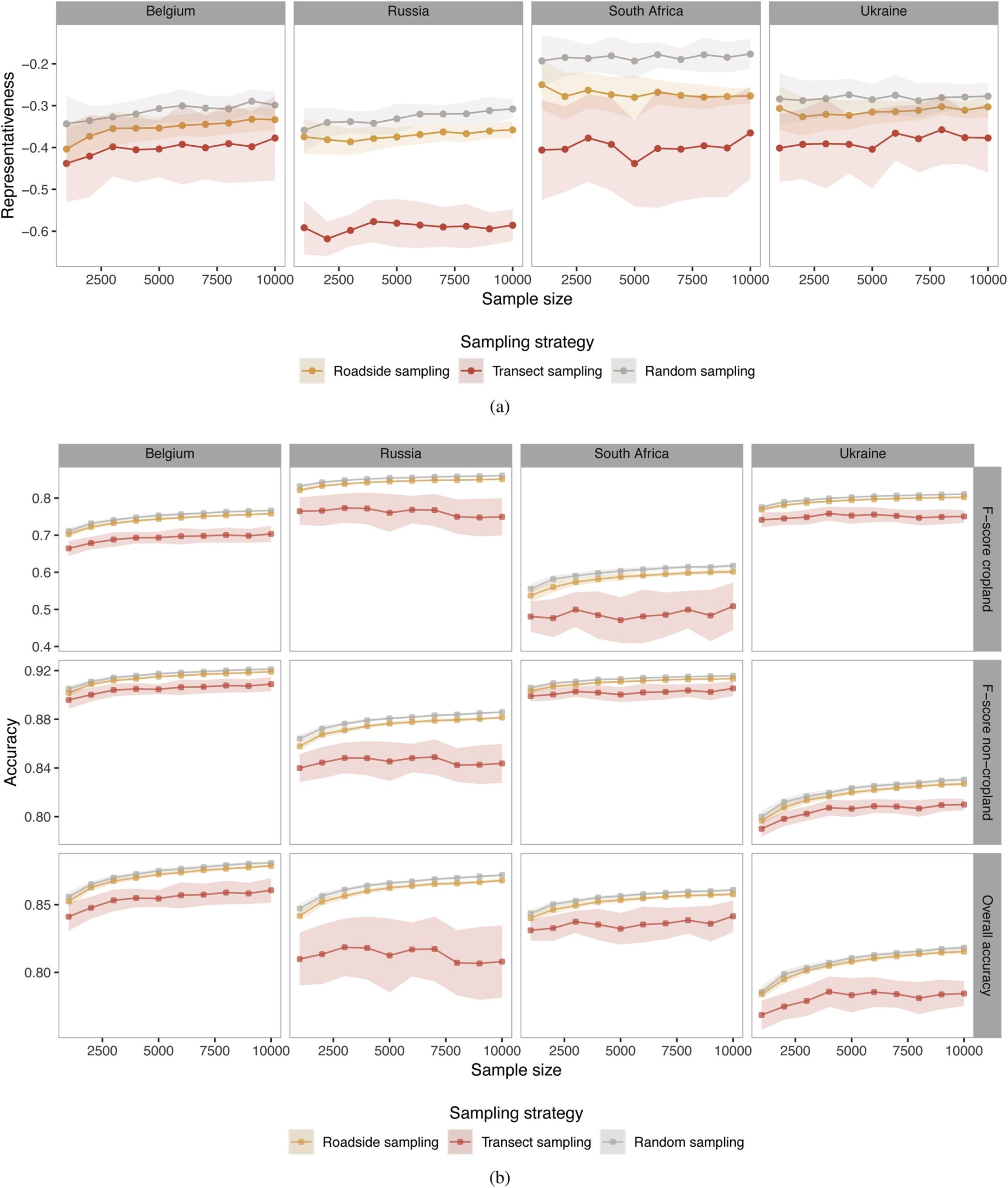
One example is the windshield survey, which was tested along with random and transect sampling schemes in Belgium, Russia, South Africa, and Ukraine in the framework of the Joint Experiment on Crop Assessment and Monitoring (JECAM). A sampling methodology as shown in the figure below was applied.
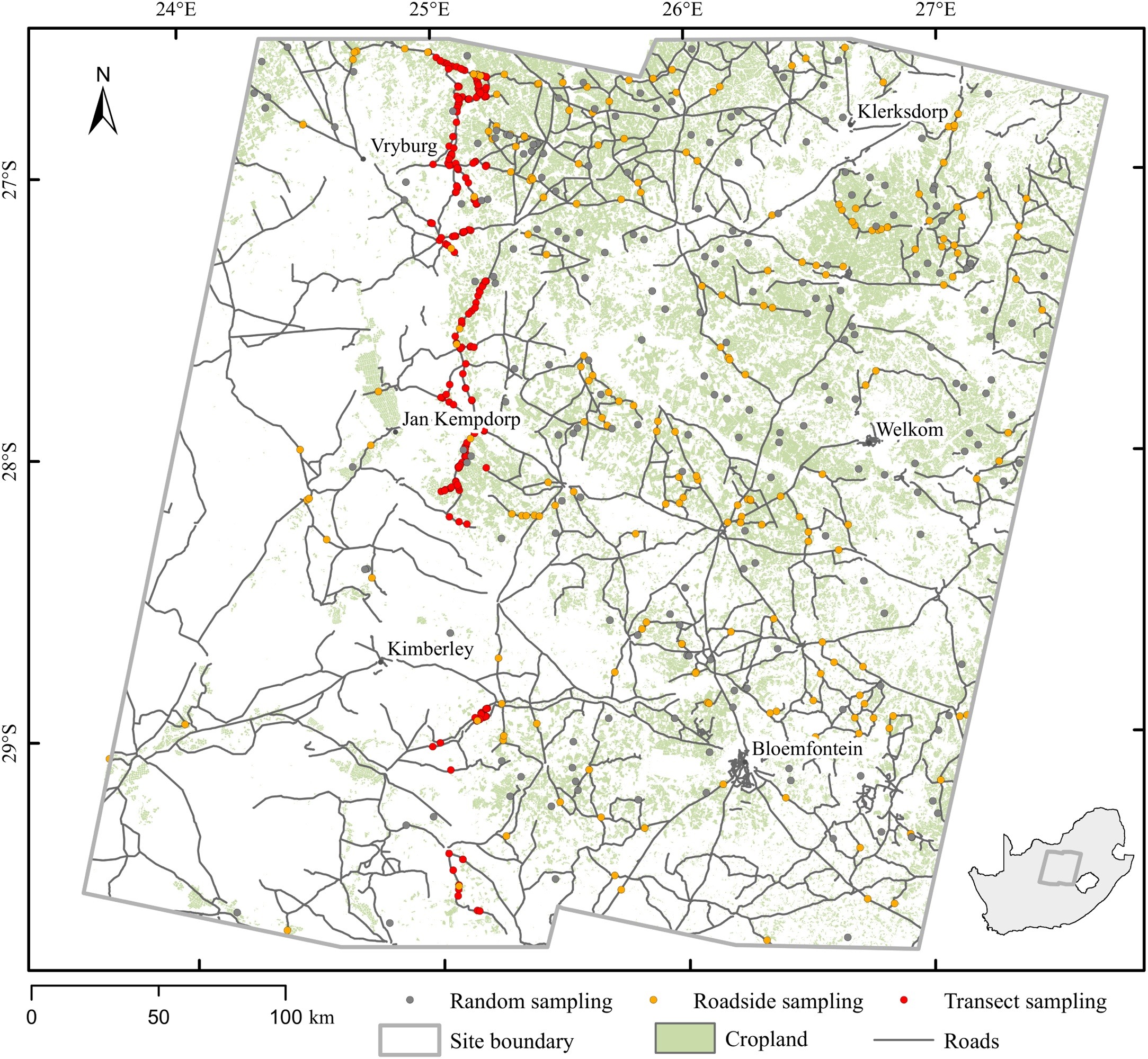
The results below show that roadside sampling did provide representative and accurate results, which critically simplifies field data collection, as roadside data collection is an easy and cheap type of survey to collect crop-type information.
The Land Use/Cover Area frame Survey (LUCAS)
Administration data is data that is collected by public authorities. It can often be used for a different purpose than it was initially collected for.
LUCAS is a land use/land cover data collection exercise of the European Union and spans its full coverage evenly. Data has been collected in 2006, 2009, 2012, 2015, and 2018, with the 2022 campaign being in preparation.
Initially designed for statistical purposes, the LUCAS data collection protocol was complemented by a Copernicus module for the first time in 2018, which corresponds to the Copernicus satellites’ spatial resolution of up to 10 m and can be used for agricultural applications like crop type mapping with Sentinel-1 imagery.
Crowdsourcing
Crowdsourcing refers to the creation of data by a large group of non-professionals. It can be active crowdsourcing, where the crowd is asked to collect specific information. Passive or opportunistic crowdsourcing means that people share information without knowing what the data is used for (see the paper from Minet et al. (2017)).
An example of both active and opportunistic crowdsourcing was the campaign #YellowFlowersEU, where people were asked to share pictures of flowering rapeseed in 2018. Citizens, scientists, farmers, and photographers contributed to a database with rapeseed flowering dates across the EU by posting pictures of yellow flowers on Twitter.
Farmer’s data
Farm management apps can offer the possibility to share data and provide in-situ information that can potentially be used in combination with remote sensing data. However, the question of data ownership can be a hindrance: Who owns and can share the data? The farmer, the platform provider, or the equipment provider?
The CEOS Cal/Val working group has assembled a repository with the scientific literature on the calibration and validation of good practices, guidelines, and standards for specific topics here (d’Andrimont, 2019; d’Andrimont et al., 2021; Defourny, 2019; Gallego & Delincé, 2010).
Credit
This topic was created with the help of learning materials that were kindly provided by:
– EO College: Land in Focus – Basics of Remote Sensing
– The European Space Agency (ESA) 9th Advanced Training Course on Land Remote Sensing with the focus on Agriculture
Sources and further readings
Sources
Congalton, R. G. (1991). A review of assessing the accuracy of classifications of remotely sensed data. Remote Sensing of Environment, 37(1), 35–46. https://doi.org/10.1016/0034-4257(91)90048-B
d’Andrimont, R. (2019, September 20). Novel In-Situ Collection Approaches for Agricultural EO Applications. 9th Advanced Training Course on Land Remote Sensing: Agriculture, Louvain-la-Neuve. https://landtraining2019.esa.int/files/14_9thLTC2019_InnovativeInSitu_Dandrimont.pdf
d’Andrimont, R., Verhegghen, A., Meroni, M., Lemoine, G., Strobl, P., Eiselt, B., Yordanov, M., Martinez-Sanchez, L., & van der Velde, M. (2021). LUCAS Copernicus 2018: Earth-observation-relevant in situ data on land cover and use throughout the European Union. Earth System Science Data, 13(3), 1119–1133. https://doi.org/10.5194/essd-13-1119-2021
Defourny, P. (2019, September 18). Accuracy Assessment: Strategy for calibration/validation and accuracy metrics. 9th Advanced Training Course on Land Remote Sensing: Agriculture, Louvain-la-Neuve. https://landtraining2019.esa.int/files/07_9thLTC2019_AccuracyAssessment_Defourny.pdf
Gallego, J., & Delincé, J. (2010). The European Land Use and Cover Area-Frame Statistical Survey. In R. Benedetti, M. Bee, G. Espa, & F. Piersimoni (Hrsg.), Agricultural Survey Methods (S. 149–168). John Wiley & Sons, Ltd. https://doi.org/10.1002/9780470665480.ch10
Minet, J., Curnel, Y., Gobin, A., Goffart, J.-P., Mélard, F., Tychon, B., Wellens, J., & Defourny, P. (2017). Crowdsourcing for agricultural applications: A review of uses and opportunities for a farm sourcing approach. Computers and Electronics in Agriculture, 142, 126–138. https://doi.org/10.1016/j.compag.2017.08.026
Olofsson, P., Foody, G. M., Herold, M., Stehman, S. V., Woodcock, C. E., & Wulder, M. A. (2014). Good practices for estimating area and assessing the accuracy of land change. Remote Sensing of Environment, 148, 42–57. https://doi.org/10.1016/j.rse.2014.02.015
Stehman, S. V., & Foody, G. M. (2019). Key issues in rigorous accuracy assessment of land cover products. Remote Sensing of Environment, 231, 111199. https://doi.org/10.1016/j.rse.2019.05.018
Waldner, F., Bellemans, N., Hochman, Z., Newby, T., de Abelleyra, D., Verón, S. R., Bartalev, S., Lavreniuk, M., Kussul, N., Maire, G. L., Simoes, M., Skakun, S., & Defourny, P. (2019). Roadside collection of training data for cropland mapping is viable when environmental and management gradients are surveyed. International Journal of Applied Earth Observation and Geoinformation, 80, 82–93. https://doi.org/10.1016/j.jag.2019.01.002
Further reading
Methods, Guidelines & Standards. (n. d.). [Repository]. CEOS Cal/Val Portal. https://calvalportal.ceos.org/methods-guidelines-good-practices
Olofsson, P., Foody, G. M., Stehman, S. V., & Woodcock, C. E. (2013). Making better use of accuracy data in land change studies: Estimating accuracy and area and quantifying uncertainty using stratified estimation. Remote Sensing of Environment, 129, 122–131. https://doi.org/10.1016/j.rse.2012.10.031
Stehman, S. V. (2013). Estimating area from an accuracy assessment error matrix. Remote Sensing of Environment, 132, 202–211. https://doi.org/10.1016/j.rse.2013.01.016
You covered the basics of food security, food systems and food security measures.
Let’s learn how food is linked to climate, environment, society, and economy.
Discussion
-
Calibration and Validation of EO products
Sorry, there were no replies found.
The forum ‘Private: Agriculture & Livestock’ is closed to new discussions and replies.