Apply Copy

Henryk Hodam

The apply* functions (e.g. apply, apply_neighborhood, apply_dimension) employ a process on the datacube that calculates new pixel values for each pixel, based on n other pixels. Please note that several programming languages use the name map instead of apply, but they describe the same type of function.

Simplified: apply([🌽, 🥔, 🐷], cook) => [🍿, 🍟, 🍖]

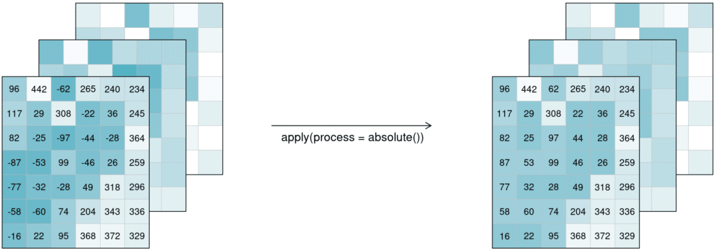
For the case n = 1 this is called a unary function and means that only the pixel itself is considered when calculating the new pixel value. A prominent example is the absolute() function, calculating the absolute value of the input pixel value.

Figure 1 – **Datacube apply unary:** 3 example tiles hold values below and above 0. after applying the process ‘absolute’, all values in the three example tiles have changed to their absolute values above 0 ().

If n is larger than 1, the function is called n-ary. In practice, this means that the pixel neighborhood is taken into account to calculate the new pixel value. Such neighborhoods can be of spatial and/or temporal nature. A spatial function works on a kernel that weights the surrounding pixels (e.g. smoothing values with nearby observations), a temporal function works on a time series at a certain pixel location (e.g. smoothing values over time). Combinations of types to n-dimensional neighborhoods are also possible.

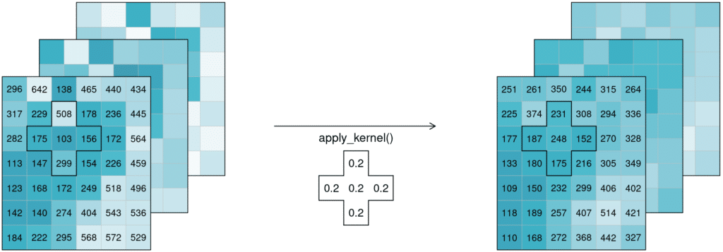
In the example below, an example weighted kernel (shown in the middle) is applied to the cube (via apply_kernel). To avoid edge effects (affecting pixels on the edge of the image with less neighbours), a padding has been added in the background.

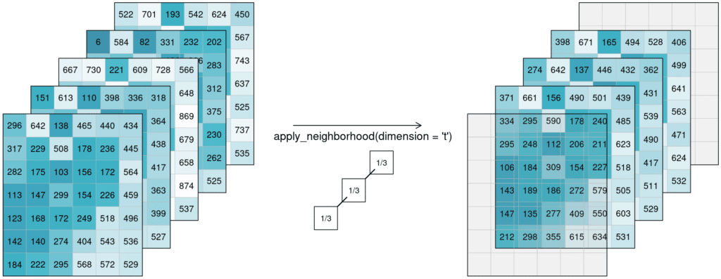
Figure 2 – **Datacube apply spatial kernel:** Three example tiles hold some values with a lot of variance. A spatial kernel (a cell plus it’s 4 direct neighbours) is applied to all pixels, and the result appears to be spatially smoothed, with less variance ().

Of course this also works for temporal neighbourhoods (timeseries), considering neighbours before and after a pixel. To be able to show the effect, two timesteps were added in this example figure. A moving average of window size 3 is then applied, meaning that for each pixel the average is calculated out of the previous, the next, and the timestep in question (t_n-1, t_n and t_n+1). No padding was added which is why we observe edge effects (NA values are returned for t₁ and t₅, because their temporal neighbourhood is missing input timesteps).

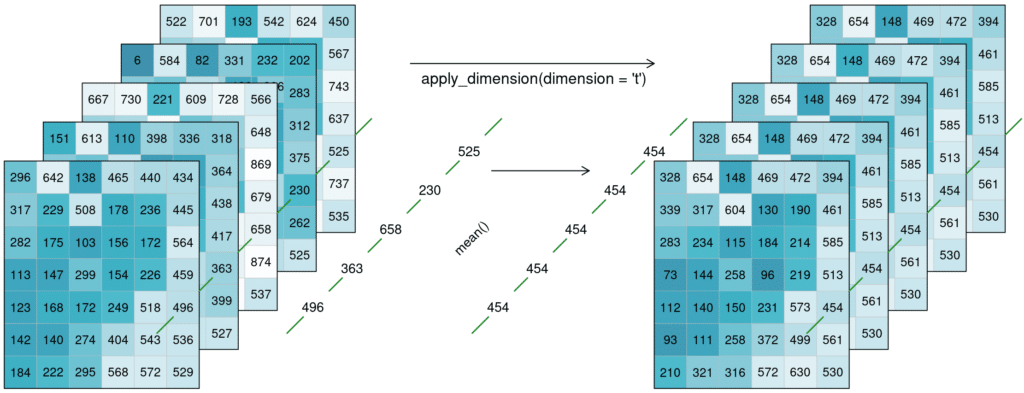
Figure 3 – **Datacube apply temporal moving average:** Smoothing is applied to 5 example tiles by calculating the mean of 3 timesteps of every single pixel. The resulting tiles for the timestamps look much more alike ().

Alternatively, a process can also be applied along a dimension of the datacube, meaning the input is no longer a neighbourhood of some sort but all pixels along that dimension (n equals the complete dimension). If a process is applied along the time dimension (e.g. a breakpoint detection), the complete pixel timeseries are the input. If a process is applied along the spatial dimensions (e.g. a mean), all pixels of an image are the input. The process is then applied to all pixels along that dimension and the dimension continues to exist. This is in contrast to reduce, which drops the specified dimension of the data cube. In the image below, a mean is applied to the time dimension. An example pixel timeseries is highlighted by a green line and processed step-by-step.

Figure 4 – **Datacube apply dimension time:** The mean of all 5 timesteps is calculated for every single pixel. The resulting 5 tiles look exaclty the same, as they have been averaged ().

Learn how to use Apply operators with this interactive exercise:

Exercise

More Information

View: for more information and links to interesting material.