

Learning objectives of this topic
- Introduction to the concept of Analysis-Ready Data
- Understand the differences between SAR product levels
- Learn about the important steps in the preprocessing of SAR imagery
- Work with SAR data in SNAP
Raw vs. Analysis-Ready Data (ARD)
In this topic we will take a closer look into the preprocessing of radar data and how the preprocessing workflow differs from the one that is used for optical data sets. The aim of preprocessing synthetic aperture radar (SAR) data, is the improvement of input information in different ways. In order to analyse the data sets reliable, the ‘raw’ data needs to be altered to: suppress noise, enhance product features and remove/minimize geometric distortions.
A term that is often used nowadays is Analysis-Ready Data (ARD) and is described by the Committee on Earth Observation Satellites (CEOS) as ‘satellite data that have been processed to a minimum set of requirements and organized into a form that allows immediate analysis without additional user support and interoperability with other datasets both through time and space’. By finding standardised ways of preprocessing SAR data, every interested scientist and/or decision maker, the entry boundary towards microwave image analysis is significantly lowered, and scientific work put to a comparable standard.
If you want to learn about the ARD concept in more detail, we recommend reading a paper by John Truckenbrodt et al. (2019).
Product levels
Similarly to what was described earlier in the preprocessing of optical data, product levels also exist for SAR data. How these differ and what characterizes them can be found below (exemplary for Sentinel-1 C-Band data).
Sentinel-1 Product Levels
Radar images are available at different processing levels. That means that a certain amount of pre-processing has already been conducted by the data provider in each product level. It is important to know which processing steps have been done at each level before ordering the data. For many users it is advantageous to order high processing levels to reduce the effort of working with the data. For others, especially scientific users, it is desirable to order data as close to the RAW data as possible to enable customized processing.
If you are interested in learning about the Sentinel-1 processing levels, click the ‘Show More’ button and discover the product levels of Sentinel-1, as described by the Sentinel-1 Product level documentation.
Show More

Inlcuded | Not included
Level 0
The SAR Level-0 products consist of compressed and unfocused SAR raw data. Level-0 products are the basis from which all other high-level products are produced. For the data to be usable, it will need to be decompressed and processed using focusing software.
Level-0 data includes noise, internal calibration and echo source packets as well as orbit and altitude information.
Level-0 products are stored in the long-term archives. They can be processed to generate any type of product during the mission lifetime and for 25 years after the end of the space segment operations.
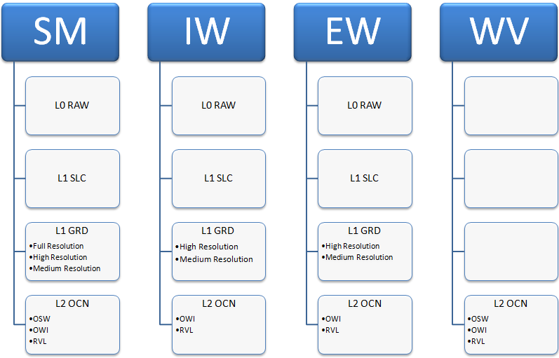
Level-0 products are available to data users for only the SM, IW and EW modes.
Level 1
Level-1 focused data are the generally available products intended for most data users. The Level-0 product is transformed into a Level-1 product by the application of algorithms and calibration data to form a baseline engineering product from which higher levels are derived.
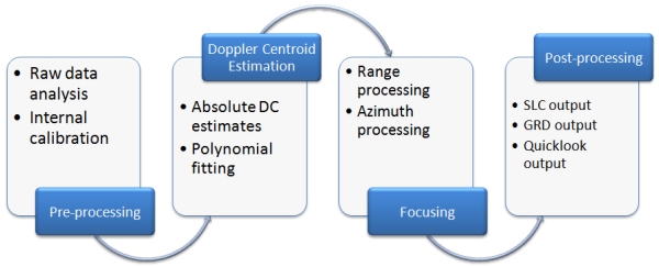
The processing involved to produce Level-1 data products includes pre-processing, Doppler centroid estimation, single look complex focusing, and image and post-processing for generation of the SLC and GRD products as well as mode specific processing for assembling of multi-swath products.
Level-1 products can be either Single Look Complex (SLC) or Ground Range Detected (GRD). Each acquisition mode can potentially generate Level-1 SLC and GRD products. GRD resolutions will depend on the mode and the level of multi-looking.
Single Look Complex
Level-1 Single Look Complex (SLC) products consist of focused SAR data, geo-referenced using orbit and altitude data from the satellite, and provided in slant-range geometry. Slant range is the natural radar range observation coordinate, defined as the line-of-sight from the radar to each reflecting object. The products are in zero-Doppler orientation, where each row of pixels represents points along a line perpendicular to the sub-satellite track.
The products include a single look in each dimension using the full available signal bandwidth and complex samples (real and imaginary) preserving the phase information. The products have been geo-referenced using the orbit and altitude data from the satellite and have been corrected for azimuth bi-static delay, elevation antenna pattern and range spreading loss.
Ground Range Detected
Level-1 Ground Range Detected (GRD) products consist of focused SAR data that has been detected, multi-looked and projected to ground range using an Earth ellipsoid model such as WGS84. The ellipsoid projection of the GRD products is corrected using the terrain height specified in the product general annotation. The terrain height used varies in azimuth, but is constant in range.
Ground range coordinates are the slant range coordinates projected onto the ellipsoid of the Earth. Pixel values represent detected magnitude. Phase information is lost. The resulting product has approximately square resolution pixels and square pixel spacing with reduced speckle at a cost of reduced geometric resolution.
Level 2
Level-2 consists of geolocated geophysical products derived from Level-1. Level-2 Ocean (OCN) products for wind, wave and currents applications may contain the following geophysical components derived from the SAR data:
- Ocean Wind field (OWI)
- Ocean Swell spectra (OSW)
- Surface Radial Velocity (RVL).
The availability of components depends on the acquisition mode. The metadata referring to OWI are derived from an internally processed GRD product, the metadata referring to RVL (and OSW, for SM and WV mode) are derived from an internally processed SLC product.
A (rough) workflow for preprocessing Level-1 data
The accordion items below describe essential steps for the preprocessing workflow of Synthetic Aperture Radar (SAR) data. However, keep in mind that these steps may differ between sensors and/or product levels.
1. Orbit File Application
As a first step, we can apply an orbit file to our SAR products. By doing so, a relationship between the coordinates of the image with the actual ground location/coordinates is drawn. The effect of this connection is a significant improvement of the accuracy. In the case of Sentinel-1, the orbit information is generated on-board, to deliver products faster. However, in order to improve orbit information, these positions are later refined by the Copernicus Precise Orbit Determination (POD) Service. The orbit files are, in the case of Sentinel-1, automatically downloaded by software packages like SNAP.
2. Radiometric Calibration
In this process, the original image pixel values, which are derived as digital numbers (DNs) are converted into actual radar backscatter. This means, that the data is manipulated in a way that provides imagery with pixel values that can be directly related to the radar backscatter of the scene. This can be achieved by changing the scaling, which is introduced by a given sensor and transfer it to a scaling range as desired. As a result of the radiometric calibration, the data set values are given as a geophysical measurement unit. The unit used to express the radiometrically calibrated SAR data is σ0.

3. De-Bursting
SAR scenes occasionally consist of multiple swaths (parts of flight strips). In the case of Sentinel, the antenna beam switches between adjacent sub-swaths, creating bursts of data. Through the synchronization (or merging) of these swaths, a single image is generated, enabling much easier data analysis and interpretation.

4. Multilooking
The multilooking is an optional step, that can help in the image interpretation. As a filtering algorithm it applies spatial averaging in order to create imagery with standardized pixel sizes. Some multilooking procedures however, reduce the image resolution, which requires compromises between spatial detail and noise reduction (radiometric resolution).
5. Speckle Filtering
In lesson two, you have learned about the origins of speckle and how it affects the interpretation of microwave imagery. The effects that are related to the fact that each scatterer in an image cell returns a vector of constant amplitude, but an arbitrary phase, leading to the speckle effect. Speckle filtering is a very important step in the preprocessing chain of SAR imagery. Contrary to the multilooking, speckle filters mostly do not reduce spatial detail. The type of filter that is used to remove speckle effects strongly depends on the application and the study site (e.g., urban areas vs. forests).
6. Terrain Correction
The terrain correction consists of two processes: Radiometric Terrain Flattening (RTF) and Geocoding.
RTF utilizes digital elevation model (DEM) information to remove radiometric distortions, which originate from the geometry of the image. This ‘removal’ process normalizes the physically meaningful backscatter values with respect to the slopes in the respective area. An example of the application of RTF is given below.
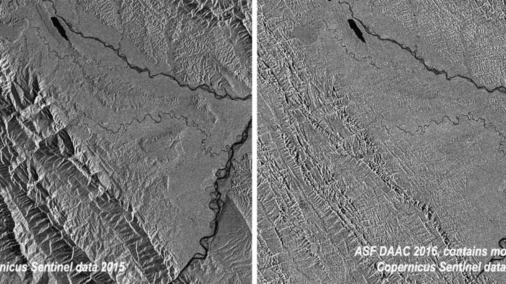
If you want to learn about this in more detail, we recommend reading a paper by David Small (2011).
The geocoding, which is also part of the terrain correction, is a transformation of coordinates, from SAR coordinates into an orthogonal geographic map projection. This is achieved by using (again) a DEM, which is used to remove common geometric effects such as shadow, layover or foreshortening. This step finally connects an image with a geographic coordinate system and makes it geographically relatable with auxiliary data sets.
7. Value Conversion
In a last step of the preprocessing, you can convert the linearly-scaled backscatter values (σ0) into a commonly used unit to describe backscatter intensities, decibels (dB). The conversion is desirable because it stretches the pixel values differently. In the image below, you can see the backscatter in the linear scale leads to the majority of values being located in the lowest region of the data range.
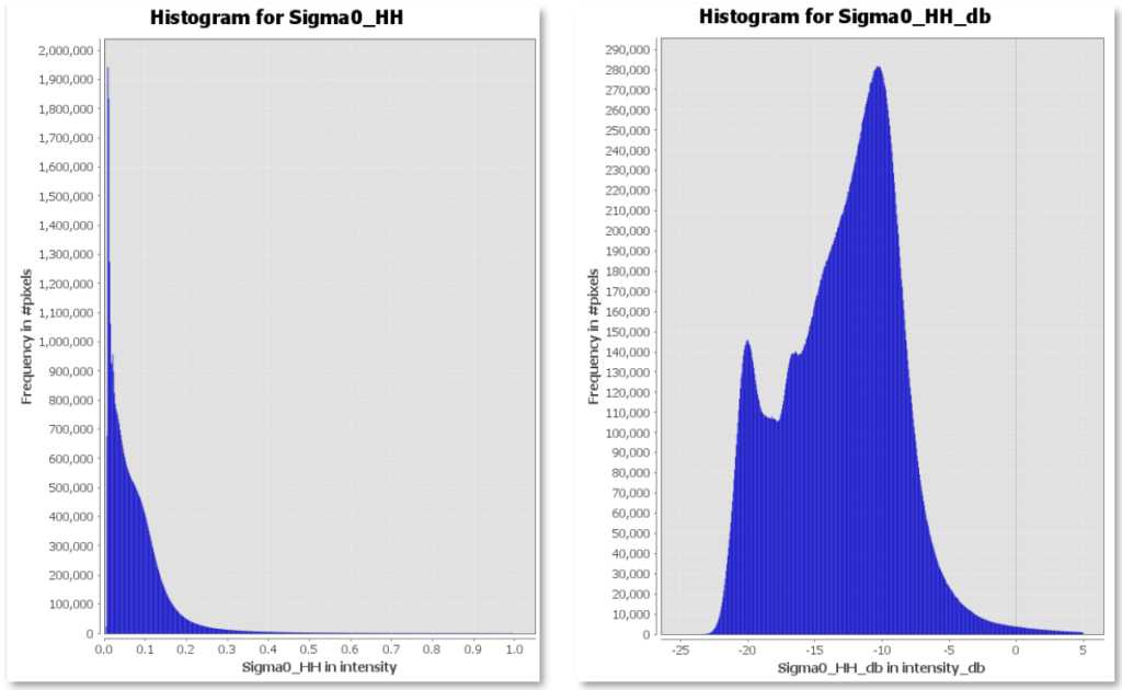
When converted into the decibel, the values are logarithmic. The log function leads to more contrast in the resulting image, as stronger backscatter values shift towards the mean and darker values get stretched stronger.
Optional practical: Working with SAR data
What is SNAP?
ESA’s Sentinel Application Platform (SNAP) is a set of toolboxes, developed for the processing and analysis of Earth observation data.
The following video tutorial gives you an introduction into the usage of the Sentinel-1 toolbox.
Hands-on: SAR data
1) Download SNAP
You can either download SNAP from the link above or use the direct links for your operating system below.
2) Download sample data
You can download some sample data below:
3) Watch the tutorial video and get your hands on some Sentinel-1 data

By loading the video, you agree to YouTube’s privacy policy.
Learn more
Sources & further reading
Braun, A. & Veci, L. (2021). Sentinel-1 Toolbox. SAR Basics Tutorial. <http://step.esa.int/docs/tutorials/S1TBX%20SAR%20Basics%20Tutorial.pdf>.
Jensen, J.R. (2007²). Remote Sensing of the Environment. An Earth Resource Perspective. Upper Saddle River, USA: Pearson Prentice Hall.
Schowengerdt, R.A. (2007³). Remote Sensing. Models and Methods for Image Processing. San Diego, USA: Academic Press.
Truckenbrodt, J., Freemantle, T., Williams, C., Jones, T., Small, D., Dubois, C., Thiel, C., Rossi, C., Syriou, A. & Guiliani, G. (2019). Towards Sentinel-1 SAR Analysis-Ready Data: A Best Practices Assessment on Preparing Backscatter Data for the Cube. In: Data (4, 93). doi:10.3390/data4030093.
Werner, C., Strozzi, T., Wegmüller, U. & Wiesmann, A. (2002). SAR Geocoding and Multi-Sensor Image Registration. Gamma Remote Sensing AG.
Woodhouse I.H. (2006). Introduction to Microwave Remote Sensing. Boca Raton, USA: Taylor & Francis Group.