
Learning objectives of this topic
- Recognize the major error sources in the RS processing chain and understand their effects
- Understand the principles of RS product validation
- Know best practices in the collection of validation data
Prerequisites
- Geometric correction/registration
- Atmospheric correction
- RS products (i.e. surface reflectance, thematic products like LAI, land cover)
Introduction: General Accuracy Assessment
The following terms and metrics are not limited to Remote Sensing but are used whenever the quality of a measurement or prediction must be quantified.
Principles of Validation
Remote Sensing is an indirect technique to measure or quantify the studied objects. Therefore, errors during the estimation process are inevitable. Error assessment or validation is typically performed with regard to an independent measurement of the target quantity. Independence means for example that the measurement was taken with another instrument or by applying another, more robust method. Usually, these validation measurements are also expected to have a higher quality than the RS derived estimates. Specifically for Remote Sensing the term ground truth is used to talk about these measurements.
Accuracy and precision
In everyday language, accuracy and precision both relate to quality and may be used as synonyms. In remote sensing (and other scientific disciplines), they have specific meanings:
Accuracy refers to the distance of a measurement (or prediction) to the true value. It can also be referred to as trueness. An accurate measurement produces results that are close to the true value.
Precision refers to the repeatability or reproducibility of a measurement. It refers to the spread that occurs if the measurement (or prediction) is repeated under the same conditions. A precise measurement produces results that are close to each other, no matter their distance from the true value.

By loading the video, you agree to YouTube’s privacy policy.
Learn more
Quality metrics
For validation purposes many quality indicators or metrics exist. All of them are meant to make the error assessment quantifiable and objective. They are used in scientific publications and reports to allow comparing different RS products with each other. The error metric that should be used to assess the quality of a RS product depends first on its type: interval and ratio scale variables like reflectance or Leaf Area Index require different metrics than nominal and ordinal scale variables like land cover. Error assessment for nominal and ordinal scale variables, important for land cover, and are discussed in the classification topic.
Additionally, quality metrics have properties that are important to understand to interpret them. Here are two examples:
R2
R2 is the correlation coefficient of a linear regression: treat the ground truth as independent and the RS product as dependent variable. Therefore, R2 only expresses how much the relationship between ground truth and RS product is following a (curvi-) linear relationship. This quality metric should better be used for explorative studies. This could for example be when using a new vegetation index to predict LAI.
Root Mean Square Error (RMSE)
The RMSE is a measure for the accuracy of a RS product, i.e. the distance of RS predictions from the corresponding ground truth measurements. It is defined as:
RMSE=\sqrt{\frac {\sum(\hat{x}_i - x_i)^2} n}It should be used when comparing metrics that should by definition be same quantities. For example, if Leaf Area Index ( LAI in m2/m2) is derived from RS data it can be compared to ground truth LAI data with the RMSE. The RMSE has the same physical unit as the RS product and the ground truth. It should be noted that the RMSE weights large errors heavier than smaller errors because of the square. Also, positive (overestimation) and negative (underestimation) errors have the same impact on RMSE.
These are just two quality metrics, for a further explanation you can see the resources below.
Surface Reflectance
Surface reflectance is a basic product in remote sensing and starting point for many applications
Still, there are several error sources contributing to the “measured” surface reflectance:
- Sensor calibration
- Atmospheric correction
The following clip provides more detail on how surface reflectance is measured, the importance of validation sites, and recent trends in surface reflectance validation.
By loading the video, you agree to YouTube’s privacy policy.
Learn more
Validation of Derived Products
Though as a user you might not have to do accuracy assessments yourself, it is important to understand how it is done and what that might mean for you when you are using satellite products and data.
This final clip focuses on the validation of remote sensing derived products, using the example of Leaf Area Index (LAI).
By loading the video, you agree to YouTube’s privacy policy.
Learn more
Tutorial
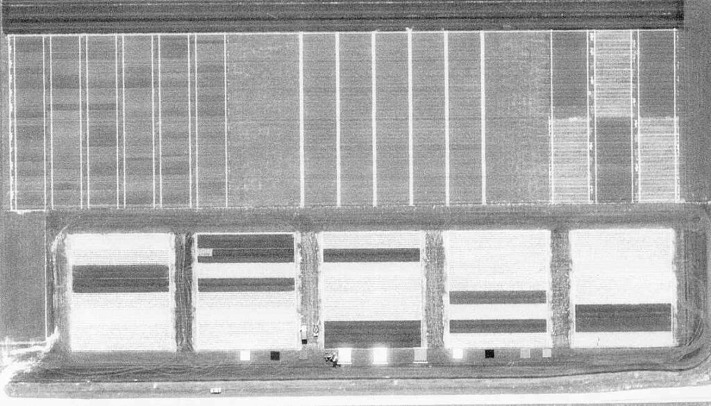
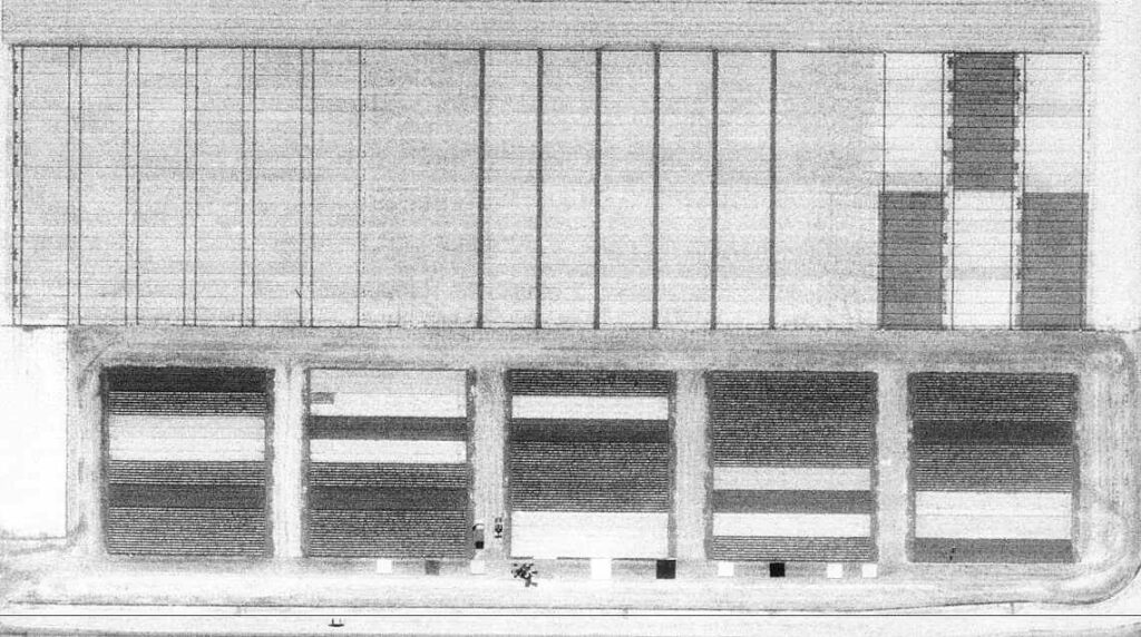
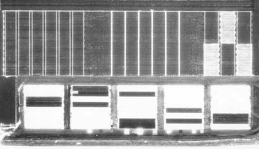
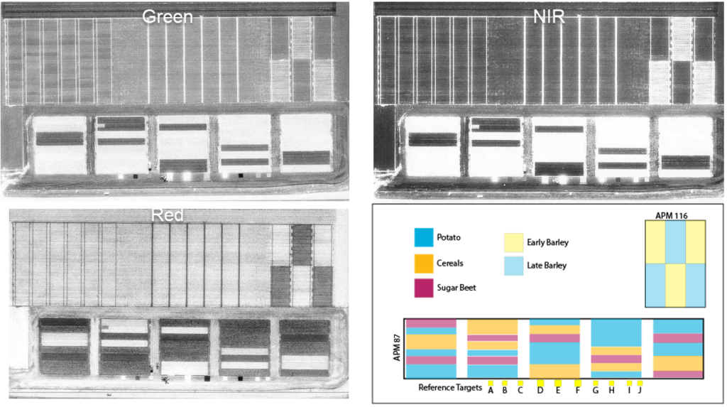
The remainder of this topic is a practical exercise where you will first derive reflectance’s from aerial images, then validate your calibration by comparing the derived values to ground truth data. This tutorial is run in two parts, first you will evaluate the digital pixel values (DN) in three black-and-white images corresponding to green, red and near infrared bands shown below.
Data Download
You can download the PDF of the tutorial and the excel file needed to complete the calculations below.
Exploring Reflectance
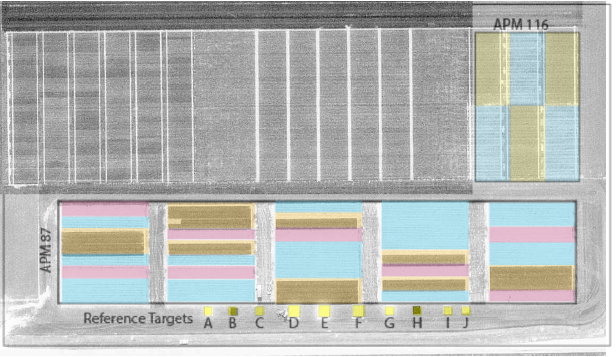
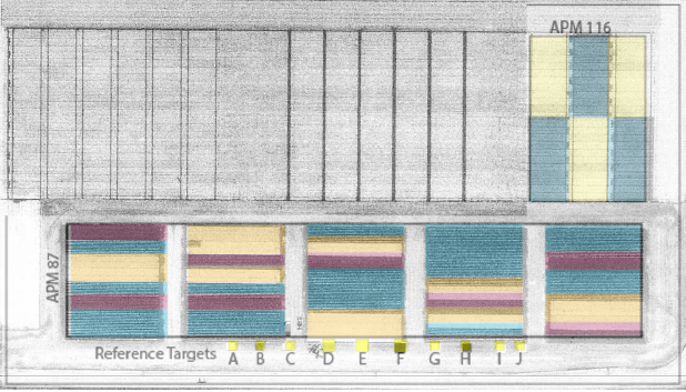
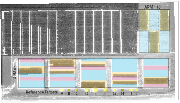
The reference targets consist of 10 different surfaces, of which the reflectances are known and which can be used for calibrating the images. They are visible on the images as the small squares below the plots. APM 87 is a rotation trial, in which different crops occur. APM 116 is a barley trial with amongst others 2 different sowing dates: early crop and late crop.
Study the three images, are the bright areas soil or vegetation?
The images have been processed such that the digital pixel values (numbers) (DN) are linearly related to the actual reflectance factor (R):
R = a + b*DP
In the three images below you can hover over the different fields and reference targets, a pop up will appear with the DN. You can also click on the buttons below to open the images in a separate page. We will be using the DN derived from these images to fill in the Excel sheet for the calibration, validation, and crop monitoring sections.
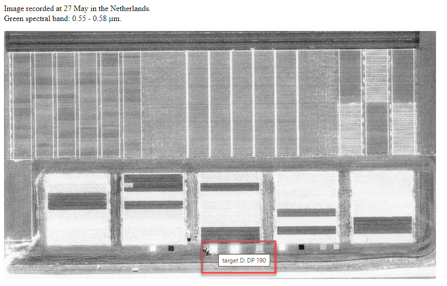
When you hover your cursor on top of a reference target or a field for a few seconds a pop-up will give you the digital number DN, it will appear both in a pop-up (highlighted in red in the image on the left).
Determine the digital pixel values (DN) for the reference targets A-F for each of the three images. Put these values in DN column of the sheet “Linear Regression” in the provided Excel.
The following table provides the actual reflectance factor (R) for the reflectance targets. The values range from 0, representing no reflectance, to 1, with all incoming light being fully reflected. Add them to the Excel sheet “Linear regression” as well. The values should turn green if you added them correctly.
As you fill in this sheet, graphs will be generated for the Green, Red, and NIR bands. You can look at the sheets Green- Red- and NIR- graph. An R2 value will also appear.
| Target | Green band | Red band | NIR band |
| A | 0.302 | 0.531 | 0.7 |
| B | 0.032 | 0.033 | 0.198 |
| C | 0.079 | 0.065 | 0.539 |
| D | 0.248 | 0.255 | 0.264 |
| E | 0.601 | 0.601 | 0.6 |
| F | 0.107 | 0.117 | 0.118 |
Validation
For the next section, go to the Excel sheet “2. Validation”.
Fill in the pixel values for reference targets G-J.
The Pixel Values (DN) of targets G and H are a bit outside of the range covered by targets A-F. This means we are extrapolating for our validation. Do you foresee any issues with this?
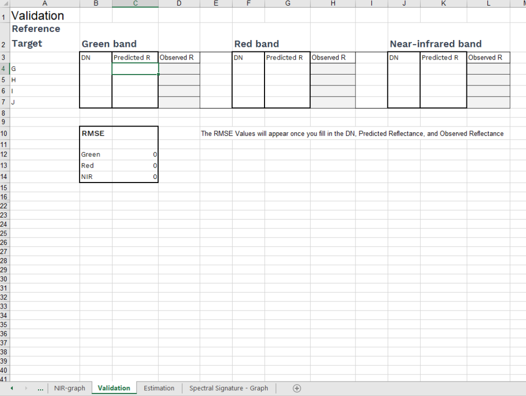
From the graphs produced in the previous step, find the reflectance values (R) for the reflectance targets, these are your predicted reflectance’s. Fill these values into the “predicted reflectance” column in sheet “2. Validation” sheet.
Your values will be compared to the true reflectance values.
Look at the RMSE for the three bands
What are the units of RMSE? Are these values acceptable for the bands?
| G | 0.450 | 0.640 | 0.750 |
| H | 0.012 | 0.015 | 0.025 |
| I | 0.097 | 0.295 | 0.570 |
| J | 0.115 | 0.135 | 0.550 |
Crop plots
Determine the pixel values (DN) for sugar beet and cereals in field trial 87. Then determine the pixel values (DN) for the early and the late crop in the barley field trial 116. You can find these values in the images in the “Exploring Reflectance Tab”
Estimate the reflectance in a green, red and near-infrared band for the 4 objects in steps 2 and 3. Using the graphs 1.1 Green, 1.2 Red, and 1.3 NIR in the excel file.
A graph of the spectral signature of these 4 objects will appear in the excel sheet titled “3.1 Spectral Signature Graph”.
In the near-infrared we can observe some darker fields within the early sown barley crop (trial 116). This is the result of differences in nitrogen nutrition. What do you expect regarding the extent of the nitrogen nutrition on these fields?
Wrap up Questions
- Why is validation important?
- What do you want to aim for when you collect validation data?
Sources & further reading
B. Alhammoud et al., “Sentinel-2 Level-1 Radiometry Assessment Using Vicarious Methods From DIMITRI Toolbox and Field Measurements From RadCalNet Database,” in IEEE Journal of Selected Topics in Applied Earth Observations and Remote Sensing, vol. 12, no. 9, pp. 3470-3479, Sept. 2019, doi: 10.1109/JSTARS.2019.2936940.
Bouvet, M.; Thome, K.; Berthelot, B.; Bialek, A.; Czapla-Myers, J.; Fox, N.P.; Goryl, P.; Henry, P.; Ma, L.; Marcq, S.; Meygret, A.; Wenny, B.N.; Woolliams, E.R. RadCalNet: A Radiometric Calibration Network for Earth Observing Imagers Operating in the Visible to Shortwave Infrared Spectral Range. Remote Sens. 2019, 11, 2401. https://doi.org/10.3390/rs11202401
Origo, N., Gorroño, J., Ryder, J., Nightingale, J., Bialek, A., 2020. Fiducial Reference Measurements for validation of Sentinel-2 and Proba-V surface reflectance products. Remote Sens. Environ. 241, 111690. https://doi.org/10.1016/j.rse.2020.111690
Willmott, C. J., & Matsuura, K. (2005). Advantages of the mean absolute error (MAE) over the root mean square error (RMSE) in assessing average model performance. Climate research, 30(1), 79-82.
In this topic you learned about Sensor accuracy. Now you are ready to move to the quiz for this lesson.
Introduction: General Accuracy Assessment
The following terms and metrics are not limited to Remote Sensing but are used whenever the quality of a measurement or prediction must be quantified.
Principles of Validation
Remote Sensing is an indirect technique to measure or quantify the studied objects. Therefore, errors during the estimation process are inevitable. Error assessment or validation is typically performed with regard to an independent measurement of the target quantity. Independence means for example that the measurement was taken with another instrument or by applying another, more robust method. Usually, these validation measurements are also expected to have a higher quality than the RS derived estimates. Specifically for Remote Sensing the term ground truth is used to talk about these measurements.
Accuracy and precision
In everyday language, accuracy and precision both relate to quality and may be used as synonyms. In remote sensing (and other scientific disciplines), they have specific meanings:
Accuracy refers to the distance of a measurement (or prediction) to the true value. It can also be referred to as trueness. An accurate measurement produces results that are close to the true value.
Precision refers to the repeatability or reproducibility of a measurement. It refers to the spread that occurs if the measurement (or prediction) is repeated under the same conditions. A precise measurement produces results that are close to each other, no matter their distance from the true value.
By loading the video, you agree to YouTube’s privacy policy.
Learn more
Quality metrics
For validation purposes many quality indicators or metrics exist. All of them are meant to make the error assessment quantifiable and objective. They are used in scientific publications and reports to allow comparing different RS products with each other. The error metric that should be used to assess the quality of a RS product depends first on its type: interval and ratio scale variables like reflectance or Leaf Area Index require different metrics than nominal and ordinal scale variables like land cover. Error assessment for nominal and ordinal scale variables, important for land cover, and are discussed in the classification topic.
Additionally, quality metrics have properties that are important to understand to interpret them. Here are two examples:
R2
R2 is the correlation coefficient of a linear regression: treat the ground truth as independent and the RS product as dependent variable. Therefore, R2 only expresses how much the relationship between ground truth and RS product is following a (curvi-) linear relationship. This quality metric should better be used for explorative studies. This could for example be when using a new vegetation index to predict LAI.
Root Mean Square Error (RMSE)
The RMSE is a measure for the accuracy of a RS product, i.e. the distance of RS predictions from the corresponding ground truth measurements. It is defined as:
RMSE=\sqrt{\frac {\sum(\hat{x}_i - x_i)^2} n}It should be used when comparing metrics that should by definition be same quantities. For example, if Leaf Area Index ( LAI in m2/m2) is derived from RS data it can be compared to ground truth LAI data with the RMSE. The RMSE has the same physical unit as the RS product and the ground truth. It should be noted that the RMSE weights large errors heavier than smaller errors because of the square. Also, positive (overestimation) and negative (underestimation) errors have the same impact on RMSE.
These are just two quality metrics, for a further explanation you can see the resources below.
Surface Reflectance
Surface reflectance is a basic product in remote sensing and starting point for many applications
Still, there are several error sources contributing to the “measured” surface reflectance:
- Sensor calibration
- Atmospheric correction
The following clip provides more detail on how surface reflectance is measured, the importance of validation sites, and recent trends in surface reflectance validation.
By loading the video, you agree to YouTube’s privacy policy.
Learn more
Validation of Derived Products
Though as a user you might not have to do accuracy assessments yourself, it is important to understand how it is done and what that might mean for you when you are using satellite products and data.
This final clip focuses on the validation of remote sensing derived products, using the example of Leaf Area Index (LAI).
By loading the video, you agree to YouTube’s privacy policy.
Learn more
Tutorial
The remainder of this topic is a practical exercise where you will first derive reflectance’s from aerial images, then validate your calibration by comparing the derived values to ground truth data. This tutorial is run in two parts, first you will evaluate the digital pixel values (DN) in three black-and-white images corresponding to green, red and near infrared bands shown below.
Data Download
You can download the PDF of the tutorial and the excel file needed to complete the calculations below.
Exploring Reflectance
The reference targets consist of 10 different surfaces, of which the reflectances are known and which can be used for calibrating the images. They are visible on the images as the small squares below the plots. APM 87 is a rotation trial, in which different crops occur. APM 116 is a barley trial with amongst others 2 different sowing dates: early crop and late crop.
Study the three images, are the bright areas soil or vegetation?
The images have been processed such that the digital pixel values (numbers) (DN) are linearly related to the actual reflectance factor (R):
R = a + b*DP
In the three images below you can hover over the different fields and reference targets, a pop up will appear with the DN. You can also click on the buttons below to open the images in a separate page. We will be using the DN derived from these images to fill in the Excel sheet for the calibration, validation, and crop monitoring sections.
When you hover your cursor on top of a reference target or a field for a few seconds a pop-up will give you the digital number DN, it will appear both in a pop-up (highlighted in red in the image on the left).
Determine the digital pixel values (DN) for the reference targets A-F for each of the three images. Put these values in DN column of the sheet “Linear Regression” in the provided Excel.
The following table provides the actual reflectance factor (R) for the reflectance targets. The values range from 0, representing no reflectance, to 1, with all incoming light being fully reflected. Add them to the Excel sheet “Linear regression” as well. The values should turn green if you added them correctly.
As you fill in this sheet, graphs will be generated for the Green, Red, and NIR bands. You can look at the sheets Green- Red- and NIR- graph. An R2 value will also appear.
| Target | Green band | Red band | NIR band |
| A | 0.302 | 0.531 | 0.7 |
| B | 0.032 | 0.033 | 0.198 |
| C | 0.079 | 0.065 | 0.539 |
| D | 0.248 | 0.255 | 0.264 |
| E | 0.601 | 0.601 | 0.6 |
| F | 0.107 | 0.117 | 0.118 |
Validation
For the next section, go to the Excel sheet “2. Validation”.
Fill in the pixel values for reference targets G-J.
The Pixel Values (DN) of targets G and H are a bit outside of the range covered by targets A-F. This means we are extrapolating for our validation. Do you foresee any issues with this?
From the graphs produced in the previous step, find the reflectance values (R) for the reflectance targets, these are your predicted reflectance’s. Fill these values into the “predicted reflectance” column in sheet “2. Validation” sheet.
Your values will be compared to the true reflectance values.
Look at the RMSE for the three bands
What are the units of RMSE? Are these values acceptable for the bands?
| G | 0.450 | 0.640 | 0.750 |
| H | 0.012 | 0.015 | 0.025 |
| I | 0.097 | 0.295 | 0.570 |
| J | 0.115 | 0.135 | 0.550 |
Crop plots
Determine the pixel values (DN) for sugar beet and cereals in field trial 87. Then determine the pixel values (DN) for the early and the late crop in the barley field trial 116. You can find these values in the images in the “Exploring Reflectance Tab”
Estimate the reflectance in a green, red and near-infrared band for the 4 objects in steps 2 and 3. Using the graphs 1.1 Green, 1.2 Red, and 1.3 NIR in the excel file.
A graph of the spectral signature of these 4 objects will appear in the excel sheet titled “3.1 Spectral Signature Graph”.
In the near-infrared we can observe some darker fields within the early sown barley crop (trial 116). This is the result of differences in nitrogen nutrition. What do you expect regarding the extent of the nitrogen nutrition on these fields?
Wrap up Questions
- Why is validation important?
- What do you want to aim for when you collect validation data?
Sources & further reading
B. Alhammoud et al., “Sentinel-2 Level-1 Radiometry Assessment Using Vicarious Methods From DIMITRI Toolbox and Field Measurements From RadCalNet Database,” in IEEE Journal of Selected Topics in Applied Earth Observations and Remote Sensing, vol. 12, no. 9, pp. 3470-3479, Sept. 2019, doi: 10.1109/JSTARS.2019.2936940.
Bouvet, M.; Thome, K.; Berthelot, B.; Bialek, A.; Czapla-Myers, J.; Fox, N.P.; Goryl, P.; Henry, P.; Ma, L.; Marcq, S.; Meygret, A.; Wenny, B.N.; Woolliams, E.R. RadCalNet: A Radiometric Calibration Network for Earth Observing Imagers Operating in the Visible to Shortwave Infrared Spectral Range. Remote Sens. 2019, 11, 2401. https://doi.org/10.3390/rs11202401
Origo, N., Gorroño, J., Ryder, J., Nightingale, J., Bialek, A., 2020. Fiducial Reference Measurements for validation of Sentinel-2 and Proba-V surface reflectance products. Remote Sens. Environ. 241, 111690. https://doi.org/10.1016/j.rse.2020.111690
Willmott, C. J., & Matsuura, K. (2005). Advantages of the mean absolute error (MAE) over the root mean square error (RMSE) in assessing average model performance. Climate research, 30(1), 79-82.