
Why do we need them
Cloud native and cloud optimized formats have been specifically designed to optimize the storage, access and processing in cloud computing environments. The main difference between cloud optimized and cloud native comes from their origin: the first are an optimized version of an existing file format whereas the latter have been designed to be efficient for a cloud usage from the beginning. These formats are tailored to leverage the scalability, flexibility, and parallel processing capabilities of a cloud infrastructure, enabling efficient handling of large-scale datasets.

By loading the video, you agree to YouTube’s privacy policy.
Learn more
“Cloud-optimized means organizing so subsets of data can be read. Ideally, the data is also compressed. Both of these factors minimize the amount of data that has to be transferred across a network.”
Characteristics
Characteristics
Cloud native and cloud optimized means mainly optimized read access, and more specifically partial and parallel reads capabilities. The main common characteristics are listed below.
Data Chunking
When working with large data files or collections, it’s often impossible to load all the data into a single computer’s memory at once. In such cases, a data chunking approach can be highly effective. By dividing the dataset into smaller chunks, the data can be processed piece by piece without exceeding the computer’s memory capacity. This approach is particularly useful for managing large datasets on a single machine and can also scale to distributed computing environments, such as cloud platforms or high-performance computing systems.
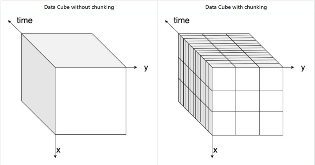
The chunk is the smallest atomic unit of a larger dataset that can be processed independently, enabling efficient data handling by dividing the dataset into manageable pieces enabling parallel processing and efficient retrieval of specific portions of the data, reducing the need to access the entire dataset.
The figure below visually explains the concept of data chunking: on the left, a three-dimensional data cube (x, y, and time) is shown without chunks, while on the right, the same data cube is displayed with chunks highlighted.
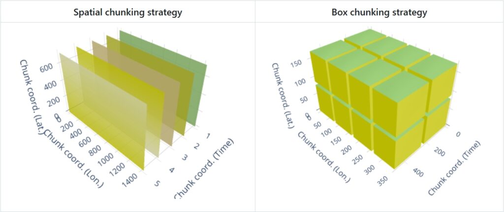
There are different ways to chunk data, depending on the nature of the dataset and the analysis requirements.
- Spatial chunking divides data based on geographical or spatial dimensions (e.g., longitude, latitude), which is ideal for geospatial datasets where the data is naturally distributed across space.
- Time-based chunking focuses on temporal dimensions (e.g., by day, month, or year), which is suitable for time-series data.
- Box chunking divides the data into fixed-size blocks (e.g., cubes or boxes), providing a balance between spatial and time-based chunking.
The choice of chunking strategy can significantly impact the efficiency of data access. Spatial chunking is optimal for spatial queries, while time-based chunking improves access to time-series data. Using the right chunking strategy can reduce the computational overhead and improve the overall performance of data processing tasks.
The image below illustrates the two most current chunking strategies:
Data Tiling
Tiling strategies are used to divide the data into smaller, manageable tiles that can be independently accessed and processed. Data tiling is similar to chunking, but specifically suited for Raster images, web maps, and tiled datasets (e.g., Web Map Tiles, Cloud-Optimized GeoTIFFs). It divides spatial data into smaller, regularly shaped regions (usually squares or rectangles) to optimize visualization and retrieval. It allows efficient loading and rendering of specific map sections without loading the entire dataset and allows access by geographic location (e.g., XYZ tiles in a web map).
Internal Indexing
These formats incorporate internal indexing structures that facilitate fast spatial and attribute queries. This enables efficient data access and retrieval operations without the need for extensive scanning or processing of the entire dataset.
Metadata Optimization
The metadata is optimized for storage and indexing, allowing for efficient access and retrieval of metadata associated with the data at once. This supports faster discovery and interpretation of data properties and characteristics.
Compression
Advanced compression techniques are often applied to reduce storage requirements while maintaining data quality.
Examples of cloud native and cloud optimized raster and multi-dimensional array formats
- Zarr is a format specifically designed for storing and accessing multidimensional arrays. It supports chunking, compression, and parallel processing, making it suitable for large-scale geospatial datasets, for example, weather data. Metadata is stored externally in data files itself. Tt can be considered the cloud evolution of netCDF, which is instead optimized for local/HPC storage.
- Cloud-Optimized GeoTIFF (COG) is an optimized version of the GeoTIFF format. It organizes raster data into chunks, utilizes internal tiling and compression, and uses HTTP range requests for efficient data access in the cloud. HTTP Range Request allows clients to request only a specific portion or range of data instead of a complete dataset.
- TileDB is a multi-dimensional, cloud-first format that supports array-based geospatial data.
Examples of cloud native and cloud optimized vector formats
- FlatGeoBuf is a cloud optimized vector data format. It is a binary encoding format for geodata and holds a collection of Simple Features.
- GeoParquet is a columnar, optimized tabular geospatial format leveraging Parquet, allowing efficient querying in cloud-based analytics.
These two formats can be used replace the Shapefile (SHP) format, which is a widely used but outdated vector data format that stores geospatial features in multiple files (.shp, .dbf, .shx). While still supported in many GIS applications, it has limitations such as file size restrictions (4GB limit), lack of support for modern cloud storage, and inefficiency in querying large datasets.
Connect the cloud native data format and it’s predecessor to it’s spatial data type:
Available Material
- Ryan Avery, Aimee Barciauskas, Development Seed, United States (2023). Technologies used to Create, Store and Access Geospatial Data in the Cloud. https://2023.ieeeigarss.org/view_paper.php?PaperNum=5306
- ESIP Talk on Cloud Native Formats: https://www.youtube.com/watch?v=ac_UKunUrNM
- FOSS4G Talk On Cloud Native Formats (Matthew Hanson)
- OGC White Paper on Cloud Native Formats (Chris Holmes, Scott Simmons):
- Cloud-Native Geospatial Foundation initiative of Radiant Earth: