Recommended prior knowledge

What you should know before viewing this presentation:

• Basics of Radar Remote Sensing
  • https://eo-college.org/resource/basics-of-sar/
  • https://eo-college.org/resource/physics/
  • https://eo-college.org/resource/sar-handbook/
• What is SAR Interferometry?
  • https://eo-college.org/resource/insar_basics/
  • https://eo-college.org/resource/introduction-to-sar-interferometry/
• What is SAR Polarimetry?
  • ​https://eo-college.org/resource/introduction-to-polarimetric-sar/
  • https://eo-college.org/resource/polsar/

Recommended prior knowledge

What you should know before viewing this presentation:

• ​What is SAR Tomography?
  • ​https://eo-college.org/resource/sar-tomography/
• How can I retrieve biomass information from SAR data?
  • https://eo-college.org/resource/biomass/

Introduction

Climate change

Source: https://pixabay.com/de/illustrations/klimawandel-die-globale-erwärmung-2063240/ (Public Domain)

Introduction

The carbon cycle is fundamental to the functioning of Earth, involving many intermeshed processes through which carbon is exchanged between the atmosphere, land, and ocean. Quantifying this global cycle is essential to understanding many of the dramatic changes taking place in the Earth system. In particular, the disturbance to the carbon cycle from the burning of fossil fuel and land-use change is the most significant driver of global change 

(IPCC, 2013)

Introduction

• Biomass is a fundamental parameter to describe the spatial distribution of carbon in the biosphere.  Therefore, biomass is a basic accounting unit for carbon (ESA, 2015).
• Recognizing these fundamental facts, ESA’s Earth Observation Programme Board selected the proposed Biomass mission to become the 7th Earth Explorer mission on 7th of May 2013.
• This presentation will provide you with a comprehensive overview of the upcoming ESA Biomass Mission. It starts with the basic intentions to design and build the system, will then list the mission objectives and requirements and provide some insights into the important technical details of the platform and the instrument. This will be followed by an overview of the mission products, algorithms to generate them, dissemination possibilities and some issues like RFI or ionospheric distortions.

1

https://www.esa.int/Newsroom/Press_Releases/ESA_s_next_Earth_Explorer_satellite

1

What is Biomass?

Given its importance for the Earth system, Biomass has been recognized as an Essential Climate Variable (ECV) by GCOS and is defined as:

A temperate forest

Source: https://pixabay.com/de/photos/wald-spring-forest-tageslicht-wald-5109810/ (Public Domain)

"Biomass is defined as mass per unit area of live or dead plant material. Unit of measure is g/m2 or multiples" (Bombelli et al., 2009).

What is Biomass?

IPCC Good Practice Guidance for LULUCF 2003 (Penman et al., 2003) divides biomass in terrestrial ecosystems into:

All living biomass above the soil including stem, stump, branches, bark, seeds, and foliage.

All living biomass of live roots. Includes fine roots (< 2 mm diameter), small roots (2 – 10 mm diameter), and large roots (> 10 mm diameter).

Dead mass

Litter

Includes all non-living woody biomass not contained in the litter, either standing, lying on the ground, or in the soil. Dead wood includes wood lying on the surface, dead roots, and stumps larger than or equal to 10 cm in diameter and greater than 1 m in length.

Above-ground biomass

Below-ground biomass

Definitions by Bombelli et al., 2009:

Includes all non-living biomass with a diameter less than a minimum diameter chosen by a given country (for example 10 cm), lying dead, in various states of decomposition above the mineral
or organic soil.

Biomass is important because:

it is a
raw material

• food
• fiber
• fuelwood

is related to vegetation structure

Biodiversity

determines rate and magnitude of autotrophic respiration

 = respiration of roots, which is another source of CO2

determines amount of carbon emitted to the atmosphere when ecosystems are disturbed

ecosystems may be disturbed due to:

• logging
• land conversion
• fire
• storms
• pests

Biomass as dry weight is about 50% carbon.

(after Houghton et al. 2009)

Forests and biomass

• Forest hold 70-90% of the terrestrial above-ground and below-ground biomass.

• Above-ground biomass accounts for 70-80 % of total forest biomass (most of it in trees).

• Above-ground biomass is vulnerable to fire, logging, land conversion (land use change), storms, pests, etc., and thus its carbon is easily released to the atmosphere.

(Houghton et al. 2009)

How can we measure biomass?

Only above-ground biomass can be measured with some accuracy at the broad scale. There are mainly four ways to measure biomass and combinations thereof (Bombelli et al., 2009):

• In-situ destructive direct biomass measurement
• In-situ non-destructive biomass estimations (using allometric equations or conversion factors)
• Derive from remote sensing data
• Vegetation Models

In-situ measurements

Tree age

• Time elapsed since germination of the seed
• Important parameter for assessing tree growth and yield
• Can be measured by counting the tree or growth rings
  • ​Tree rings may also be called annual ring as they correspond to

  • Every year of growth, which is not completely true, as the
    formation of tree rings only occurs during the vegetation period,
    which may last four to five months depending on the latitude and

    local climatic conditions.

• Can be counted at dead felled tree or with an increment borer  for
  living trees with which an increment  core is extracted from the
  tree at breast height, (Van Laar and Akça 2007).

Tree rings

Source: https://upload.wikimedia.org/wikipedia/commons/4/42/Tree_rings.jpg 
(License CC BY‐SA 2.5)

Increment borer

Source: https://upload.wikimedia.org/wikipedia/commons/3/34/Pressler_drill_5_beentree.jpg
(License CC BY‐SA 3.0)

https://en.wikipedia.org/wiki/Increment_borer

https://en.wikipedia.org/wiki/Dendrochronology#Growth_rings

1

1

2

2

In-situ measurements

Tree diameter

• In forestry, the diameter of a tree stem is used as a direct measure that, together with other variables, can be used to compute cross-sectional areas, surface area and tree volume via allometric formulas.
• Tree diameter is typically measured at breast height, abbreviated DBH (= diameter at breast height)
  • In the USA, this is a height of 4.5 feet above ground.
  • In countries using the metric system, the breast height
    is measured at 1.3 m above ground level
  • Instruments commonly used in forestry to
    measure BHD are calipers or simple measuring
    tapes

Beam caliper

Source: https://upload.wikimedia.org/wikipedia/commons/3/3b/Kluppeneinsatz.jpg
(License CC BY‐SA 3.0)

Husch et al. 2002

In-situ measurements

Tree height

• Most important vertical distance measure
• Is an ambiguous term if not clearly defined
  • Total tree height h is defined as the vertical distance along the axis of the tree between the tree top and the ground
  • Bole height hb is defined as the vertical distance along the axis of the tree between the crown point and the ground
    • Crown point is the point, where the first crown‐forming branch is located.
  • Merchantable height hm is defined as the vertical distance along the axis of the tree between the terminal position of the last usable position of the stem and the ground

(De Young 2016)

Different measures for tree height

Remote Sensing of Biomass

Further reading

• Kumar, L., Sinha, P., Taylor, S., & Alqurashi, A.F. (2015). Review of the use of remote sensing for biomass estimation to support renewable energy generation. Journal of Applied Remote Sensing, 9, 097696
• Shi, L., & Liu, S. (2017). Methods of Estimating Forest Biomass: A Review. In J.S. Tumuluru (Ed.), Biomass volume estimation and valorization for energy (p. 516). London: IntechOpen (https://www.intechopen.com/books/5393)
• Sinha, S., Jeganathan, C., Sharma, L.K., & Nathawat, M.S. (2015). A review of radar remote sensing for biomass estimation. International Journal of Environmental Science and Technology, 12, 1779-1792
• Timothy, D., Onisimo, M., Cletah, S., Adelabu, S., & Tsitsi, B. (2016). Remote sensing of aboveground forest biomass: A review Tropical Ecology, 57, 125-132

 EO -College: https://eo-college.org/resource/biomass/

Carbon Cycle & The Need for Biomass data

Atmosphere

Land

Ocean

Exchange of C as result of diffusion of CO2 across ocean surface

• The carbon cycle is a global biogeochemical cycle, where carbon (C) is exchanged between the three major reservoirs: Atmosphere, Land, Ocean.

Carbon sequestration through photosynthesis of plants

Release of carbon through respiration of plants and soils

Carbon Cycle without anthropogenic activities

Carbon Cycle & The Need for Biomass data

Atmosphere

Exchange of C as result of diffusion of CO2 across ocean surface

Carbon sequestration through photosynthesis of plants

Release of C through respiration of plants and soils

Carbon Cycle with anthropogenic activities

Release of C through burning of fossil fuels, land use change, agricultural practices, cement production

Since the beginning of the industrial revolution around 1750, humans released large amounts of greenhouse gases (CO2, CH4, N2O) to the atmosphere.

Ocean

Land

Facts and Figures

(IPCC, 2013)

• Since the start of the industrial revolution, the concentration of atmospheric CO2 increased by 40% from 278 ppm in 1750 to 390.5 ppm in 2011.
   
• The concentration of other greenhouse gases increased too – during the same time interval, CH4 increased by 150% from 722 ppb to 1803 ppb, and N2O by 20% from 271 ppb to 324.2 ppb in 2011.
   
• Current concentrations of atmospheric CO2, CH4 and N2O exceed any level measured for at least the past 800,000 years (period covered by ice cores)
   
• Furthermore, the average rate of increase of these three gases observed over the past century exceeds any observed rate of change over the previous 20,000 years.

Facts and Figures

• Global carbon budget averaged over the last half-century revealed that 82 % of the total emissions were caused by fossil CO2 emissions and 18 % by land use change (Friedlingstein et al. 2019)
   
• One-third of the CO2 released from burning fossil fuels, is absorbed by forests every year (Harris et al. 2021)
   
• Research found that the world’s forests sequestered about twice as much CO2 as they emitted between 2001 and 2019; forests provide a “carbon sink” that absorbs a net 7.6 billion metric tonnes of CO2 per year (Harris et al. 2021)

"With a very high level of confidence, the increase in CO2 emissions from fossil fuel burning and those arising from land use change are the dominant cause of the observed increase in atmospheric CO2 concentration" (IPCC, 2013, p. 467).

Facts and Figures

The net terrestrial land-atmosphere flux is not measured directly, but is inferred by subtracting the fossil fuel and net ocean-atmosphere fluxes from the observed atmospheric increase.

This inevitably causes the net land‑atmosphere flux to have the largest uncertainty amongst all the net fluxes. The land surface is found to be a net carbon sink, with uncertainty of the same order as its magnitude.

Further Information Carbon Cycle

NOAA - The Carbon cycle

https://www.noaa.gov/education/resource-collections/climate/carbon-cycle

IPCC, Climate Change 2013: The Physical Science Basis, Chapter 6: Carbon and Other Biogeochemical Cycles
https://www.ipcc.ch/report/ar5/wg1/carbon-and-other-biogeochemical-cycles/

IPCC, Climate Change 2001: The Scientific Basis, Chapter 3: The Carbon Cycle and Atmospheric Carbon Dioxide
https://www.ipcc.ch/report/ar3/wg1/the-carbon-cycle-and-atmospheric-carbon-dioxide/

Source: NOAA

Illustration of the Carbon Cycle

Global Carbon Project
https://www.globalcarbonproject.org/carbonbudget

Why do we need the Biomass Mission?

The ESA P-band Biomass mission is designed "to reduce the major uncertainties in carbon stocks and fluxes associated with the terrestrial biosphere, including carbon fluxes associated with Land Use Change, forest degradation and forest regrowth." (Quegan et al. 2021)

"The main goal of the Biomass mission is contributing to reduce the uncertainty in the worldwide spatial distribution and dynamics of forest biomass, with the final aim to improve current assessments and future projections of the global carbon cycle." (Carbone et al. 2021)

Uncertainties?

Uncertainty

Accuracy

Precision

Accuracy refers to the closeness of the measurements to a specific value and describes systematic errors, a measure of statistical bias; low accuracy causes a difference between a result and a "true" value.

Precision refers to the degree to which individual measurements vary around a central value and describe  random errors, a measure of statistical variability.
Measurements with high precision are highly reproducible as repeated measurements will reliably lead to similar results; however.

Measurements may be precise but accurate, not precise but accurate, precise and accurate or not precise and not accurate.

Uncertainties?

• National forest inventory data are the basis for annual global reports on forest resources and carbon stocks.
• In most developed countries there are operational methodologies for biomass inventories by national authorities (e.g. forest services) using different techniques (e.g. field based surveys, LiDAR, remote sensing) -each method comes with its own uncertainties.
• In most developing countries, such biomass information are uncertain or do not exist at all. This is especially unfortunate because these are the countries experiencing great changes and fast rates of deforestation.
• Furthermore, different definitions, standards, and qualities in national inventories lead to biases and uncertainties. If supra-national bodies (e.g. FAO) collect country reports (national reports/inventories) and, together with remote sensing based biomass assessments at selected sampling sites, creates global reports like the Global Forest Resources Assessment, uncertainties sum up.

(Bombelli et al., 2009)

In-situ measurements

• AGB estimated from in-situ measurements of variables using an allometric model as a function of ρ as stem wood density of the focal tree, D as trunk diameter at breast height, and H as its total height:
  
  
  
   
• To get AGB values at plot* level, tree-level AGB estimates are summed across trees and over the plot area
• Errors due to the estimation of height, wood density, and choice of the allometric model usually result in a plot-based AGB uncertainty that is non-negligible.
  • AGB is estimated with ~50% absolute error for a single tree 
  • When propagated at stand level, error is ~10% at the 1-ha scale 

(Chave et al., 2019, Chave et al., 2014, Réjou-Méchain et al. 2014)

Errors / Uncertainties

* A plot is a parcel of woodland or forest

Mission Requirements

Objectives

Geophysical Product Requirments

Level-1 Data Requirements 

ESA (2015): Biomass Mission Requirements Document, EOP-SM/1645

1

1

2

Level-1 Data: SAR data are available at different levels of processing and usability for the user, please see also Mission Products

2

Geophysical Product Requirements

1. Product Definition

(ESA 2015, p. 30)

Geophysical Product Requirements

2. Coverage

Fig. 4.1 of the Biomass Mission Requirements Document showing spatial coverage requirement of the mission 

Source: ESA Biomass Mission Requirements Document 

(ESA 2015, p. 30)

Geophysical Product Requirements

3. Spatial Resolution

4. Temporal Sampling

(ESA 2015, p. 36)

(ESA 2015, p. 36)

Geophysical Product Requirements

5. Uncertainty

-1

-1

(ESA 2015, p. 37)

Geophysical Product Requirements

6. Latency

What is latency?

Generally speaking, latency can be seen as time delay between the cause and the effect of some physical change in a system under observation.

In the context of the Biomass Mission, data latency means the time required from the data acquisition by the sensor and the availability of the products to the users. When the mission was designed, it was decided that there is no need for near-real-time processing.

(ESA 2015, p. 37)

Geophysical Product Requirements

7. Mission Duration

(ESA 2015, p. 37)

Level-1 Data Requirements

1. Observing technique and selection of frequency

2. Polarisation

(ESA 2015, p. 46)

(ESA 2015, p. 48)

Level-1 Data Requirements

3. Incidence Angle

4. Geolocation Requirements

(ESA 2015, p. 48)

(ESA 2015, p. 49)

Level-1 Data Requirements

5. Dynamic Range

6. Radiometry

(ESA 2015, p. 49)

(ESA 2015, p. 50)

6.1. Resolution and number of looks 

Level-1 Data Requirements

(ESA 2015, p. 52)

6.2. Radiometric bias and stability

(ESA 2015, p. 52)

6.3. Noise Equivalent Sigma Nought

(ESA 2015, p. 52)

Level-1 Data Requirements

(ESA 2015, p. 53)

6.4. Range and azimuth ambiguities

(ESA 2015, p. 54)

6.5. Cross Talk and Channel Imbalance

(ESA 2015, p. 54)

Level-1 Data Requirements

7. Phase Errors

(ESA 2015, p. 54)

Level-1 Data Requirements

8. Interferometric Requirements

(ESA 2015, p. 54)

Level-1 Data Requirements

9. Orbit/Mission Phases

(ESA 2015, p. 55)

Level-1 Data Requirements

9. Orbit/Mission Phases

(ESA 2015, p. 55)

9.1. Interferometric phase repeat cycle and baseline

(ESA 2015, p. 56)

Level-1 Data Requirements

9.2. Tomographic phase repeat cycle and baseline

(ESA 2015, p. 57)

Level-1 Data Requirements

9.3. Local time of the orbital node at the equator

(ESA 2015, p. 58)

Why P-band?

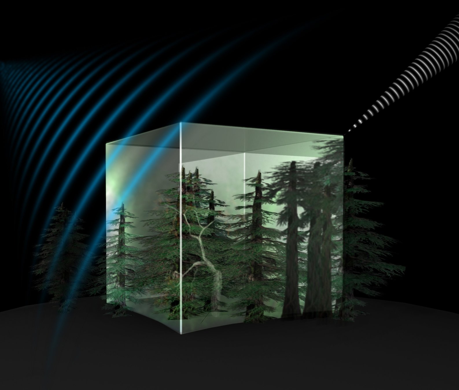
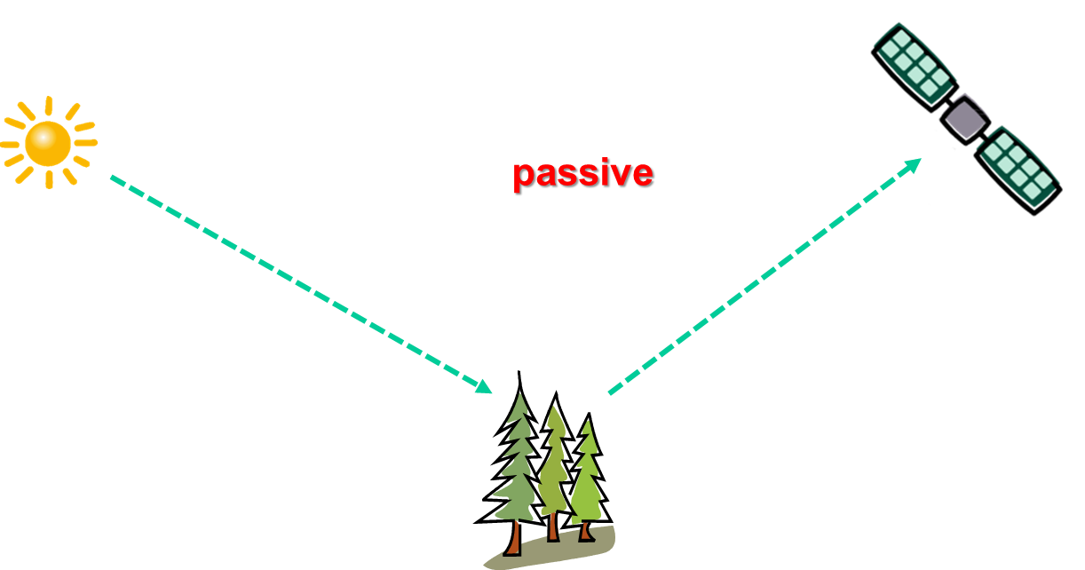
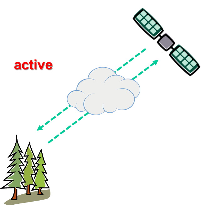
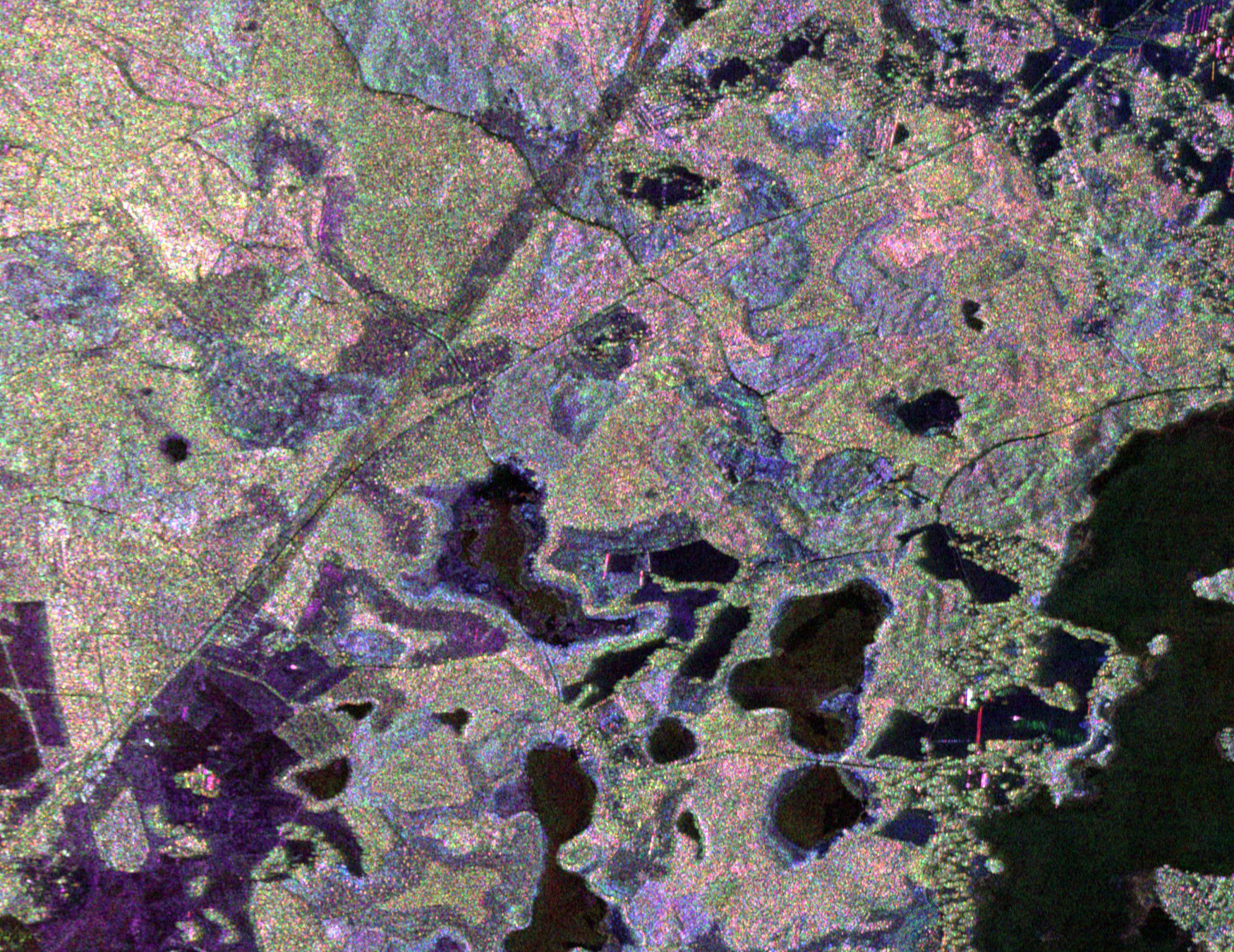
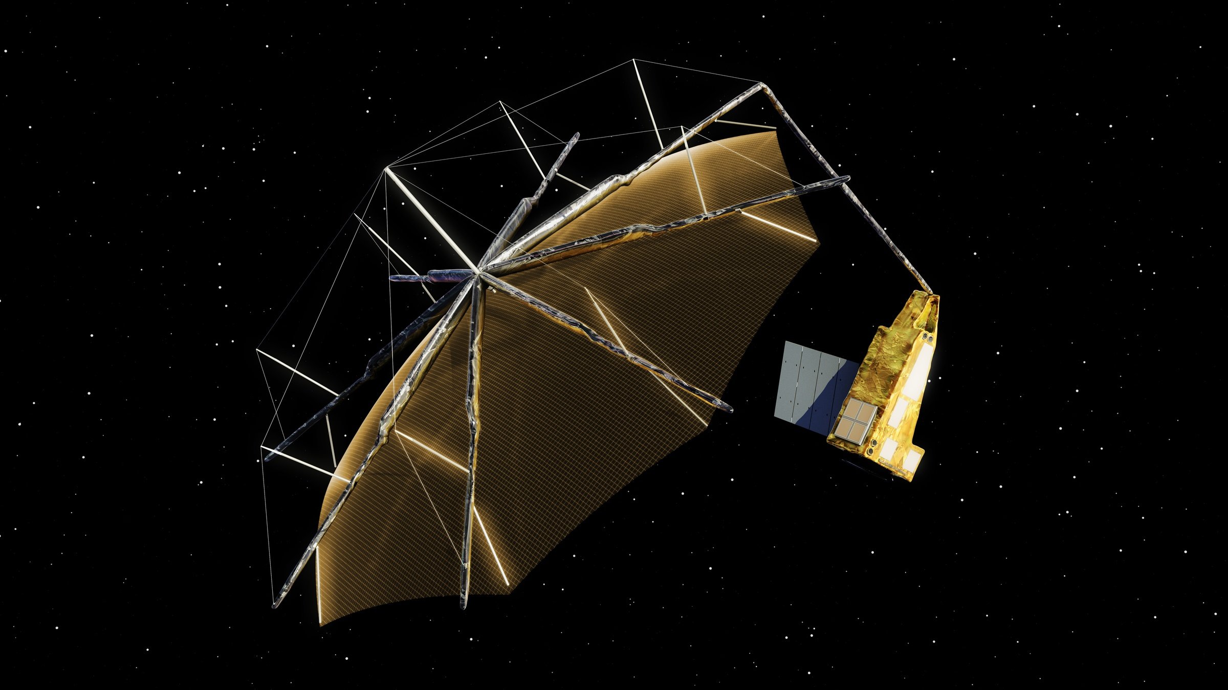
Why P-band has been selected as information carrier for the ESA Biomass Mission? Before this question is answered, we will take a closer look at radar frequency bands.

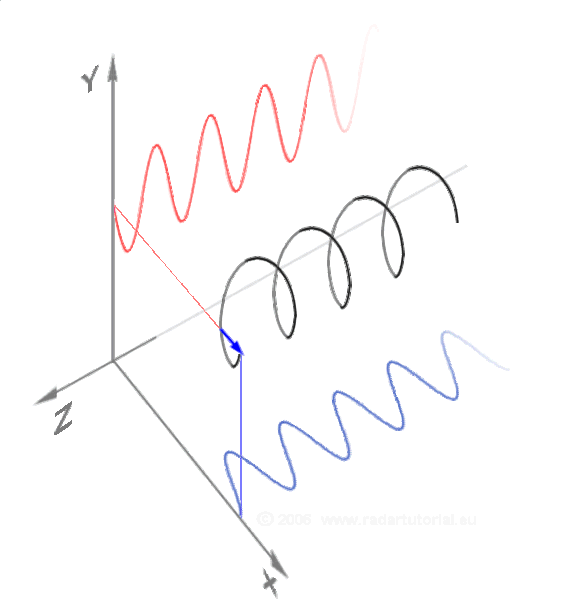
They are small sections of the electromagnetic spectrum, which integrates electromagnetic radiation at all wavelengths or frequencies. Active remote sensing techniques, like the P-band SAR Biomass Mission, are using the microwave region of the electromagnetic spectrum. This covers a wide range of wavelengths λ or frequencies f ranging from wavelengths of 1 mm (300 GHz) to 1 m (0.3 GHz).
 

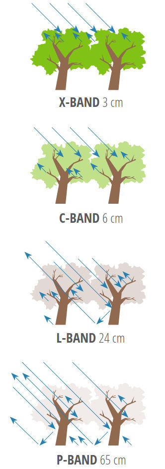
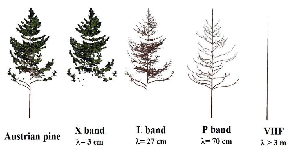
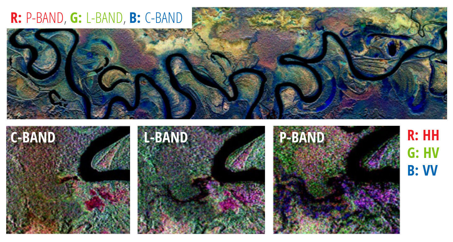
The microwave range is divided into a number of so-called radar bands, designated with a capital Latin letter.

• The ESA Biomass Satellite will be the first operational space-borne P-band Synthetic Aperture Radar (SAR)
   
• P-band
  • Radar bands defined by the International Telecommunication Union
  • Defined as electromagnetic frequency band with
    • Wavelength 30 - 100 cm or
    • Frequency 1 - 0,3 GHz
  • Sometimes P-band is also called UHF standing for Ultra High Frequency

Why P-band?

Why P-band?

P-band SAR as an active remote sensing technique using the microwave region of the electromagnetic spectrum is (almost) independent of:

• Sunlight and thus time of the day
• Weather conditions as microwaves can penetrate clouds (with some limitations)

Why P-band?

ESA SAR Earth Observation Satellite Sentinel-1 acquiring C-band SAR data through clouds

Source: https://www.esa.int/Applications/Observing_the_Earth/Copernicus/Sentinel-1/Instrument
(© ESA/ATG medialab)

• The ability to penetrate a vegetation canopy mainly depends on the used radar band = frequency of the radiation (or its wavelength)
   
• As a rule of thumb, it can be said that the larger the wavelength, the deeper the penetration depth.​

Why P-band?

(Source: The SAR Handbook
https://servirglobal.net/Global/Articles/Article/2674/sar-handbook-comprehensive-methodologies-for-forest-monitoring-and-biomass-estimation, p.216)

Sensitivity of SAR measurements to forest structure and penetration into the canopy
at different wavelengths

• The ability to penetrate a vegetation canopy mainly depends on the used radar band = frequency of the radiation (or its wavelength)
   
• As a rule of thumb, it can be
  said that ​at large wavelengths,
  only large parts of a tree
  contribute to radar
  backscatter signals.

Why P-band?

(Source: Le Toan 2007,

http://earth.esa.int/landtraining07/D3L3-LeToan.pdf)

Main scatterers at different frequencies

leaves, twigs

leaves, small branches

branches and trunk

trunk

Main scatterers:

Why P-band?

(Source: The SAR Handbook
https://servirglobal.net/Global/Articles/Article/2674/sar-handbook-comprehensive-methodologies-for-forest-monitoring-and-biomass-estimation, p.217)

Examples of SAR imagery at C-, L-, and P-band (AIRSAR) over tropical forests along the Ja River in Papua New Guinea showing differences of penetration and impacts of forest structure as SAR false color composite (HH, HV, VV) imagery.

Why P-band?

(Source: https://www.esa.int/Applications/Observing_the_Earth/FutureEO/Biomass/Measuring_forest_biomass_from_space_-_ESA_campaign_tests_BIOMASS_mission,
© ESA)

An example of a P-band SAR image recorded by the DLR E-SAR airborne instrument over Reminstorp in Sweden. Acquired in September 2010 during the BioSAR campaign.

RGB Colour Composite: R = HH, G = HV, B = VV The forest stand and site characteristics are reflected in the different tones and colours of the image.

Why P-band?

P-band radar backscatter:

• Shows highest sensitivity to biomass compared to all other frequencies that can be exploited from space
• Can penetrate the canopy in all forest biomes and interacts preferentially with the large woody vegetation elements in which most of the biomass resides
• Is more sensitive to biomass than at higher frequencies (X-, C-, S- and L-bands); lower frequencies (e.g. VHF) display even greater sensitivity but present formidable challenges for space borne SAR because of ionospheric effects
• Displays high temporal coherence between passes separated by several weeks, even in dense forest - allows use of Polarimetric interferometric SAR (PolInSAR) to retrieve forest height and use of Tomographic SAR (TomSAR) to retrieve vertical structure
• P-band is highly sensitive to disturbances of the biomass

(Quegan et al. 2019, Carbone et al. 2021)

Mission Planning

• With the Living Planet Programme (LPP) ESA developed a new strategy for Earth Observation, where Earth observation missions are divided into Earth Explorer and Earth Watch missions (Simon et al., 2006)

Earth Explorer Missions

Earth Watch Missions

Research and demonstration

User driven operational missions

• Copernicus Programme (The Sentinels)
• Cooperation of ESA with EUMETSAT

Earth Explorers

Links:

Earth Watch

Living Planet Programme

GOCE, SMOS, CryoSat, Swarm, ADM-Aeolus, EarthCare, Biomass

Mission Planning

(Source: https://www.esa.int/Science_Exploration/Space_Science/How_a_mission_is_chosen)

Typical phases on an ESA mission

The Biomass launch is expected around the end of 2023 and is planned to be a five-year mission.

Mission Planning & Preparation Timeline

March 2005

May 2006

Phase 0
Preliminary Feasibility Studies

(Source:
ESA, 2015,
Scipal et al., 2010, https://directory.eoportal.org/web/eoportal/satellite-missions/b/biomass)

Mission Planning & Preparation Timeline

January 2009

2010/2011

Presentation of the 6 Candidate Missions at a User Consultation Meeting

Subsequent down-selection of 3 Candidate Missions for a Phase-A Feasibility Study

Conduction of study; formally completed by Preliminary Requirements
Review (PRR)

(Source:
ESA, 2015,
Scipal et al., 2010, https://directory.eoportal.org/web/eoportal/satellite-missions/b/biomass)

Mission Planning & Preparation Timeline

January 2013

Extension of Phase-A studies by 6 months to address critical issues found during studies and to further consolidate the scientific dossier of the proposed candidates

Results of extension published in "Addendum to the Report for Mission Selection"

Reports for Mission Selection for the 3 Candidate Missions issued

June 2012

Earth Science Advisory Committee (ESAC) recommended implementing Biomass as the 7th Earth Explorer Mission

March 2013

(Source:
ESA, 2015,
Scipal et al., 2010, https://directory.eoportal.org/web/eoportal/satellite-missions/b/biomass)

Mission Planning & Preparation Timeline

May 2013

April 2016

ESA and Airbus Defence and Space UK signed a €229 million contract to build the next Earth Explorer: the Biomass satellite, due to begin its mission in 2021

Approval of Biomass Mission as the 7th Earth Explorer Mission in the frame of Earth Observation Envelope Programme

(Sources:
ESA 2015,
ESA, May 7 2013,"N° 13–2013: ESA’s next Earth Explorer satellite", URL: https://www.esa.int/Newsroom/Press_Releases/ESA_s_next_Earth_Explorer_satellite,
Scipal, 2017,
ESA, May 3, 2016: ”Ready to build the BIOMASS forest mission”, URL: http://www.esa.int/Our_Activities/Observing_the_Earth/Ready_to_build_the_Biomass_forest_mission,

ESA, 28 Oct 2019: "Contract seals deal for Biomass satellite’s ride into space", URL: https://www.esa.int/Applications/Observing_the_Earth/Biomass/Contract_seals_deal_for_Biomass_satellite_s_ride_into_space)

ESA and Arianspace sign Launch Contract and secure launch of ESA Earth Explorer Biomass Satellite with lift-off from French Guiana scheduled for 2022

October 2019

https://www.esa.int/Newsroom/Press_Releases/ESA_s_next_Earth_Explorer_satellite

Mission Planning & Preparation Timeline

April 2021

Biomass satellite successfully completed a suite of mechanical tests including sine vibration, acoustic, shock and clamp-band release tests.

(Source:
ESA, 28th April 2021: "Forest measuring satellite passes tests with flying colours", URL: https://www.esa.int/Applications/Observing_the_Earth/Biomass/Forest_measuring_satellite_passes_tests_with_flying_colours,
ESA, 29th October 2021: "ESA and NASA launch revolutionary open-source platform", URL: https://www.esa.int/Applications/Observing_the_Earth/ESA_and_NASA_launch_revolutionary_open-source_platform,
ESA - biomass - ESA's forest mission, URL: https://www.esa.int/Applications/Observing_the_Earth/FutureEO/Biomass)

The Biomass launch is expected around 2023 and is planned to be a five-year mission.

2023

ESA and NASA launch MAAP open-source platform

Ocotber 2021

Biomass Mission Phases

(Source: Sedehia et al., 2021)

• BIOMASS mission is designed for lifetime of 5 years
• Will consist of two phases:
  • Tomographic phase (TOM) of 1 year followed by the
  • Interferometric phase (INT)

Tomographic
Phase
(TOM)

Interferometric Phase (INT)

Commis-
sioning
Phase

launch

+

4 months

End of
planned
lifetime

end of year 1

end of year 1

end of year 2

end of year 3

end of year 4

end of year 5

duration:
12 months

Biomass Mission Phases

Biomass Mission Phases

TOM

• will last 1 year starting after commissioning phase
• during the TOM phase, 6 spatial baselines resulting in 7 SAR acquisitions for a given location will be obtained
  • For separating 3 – 4 layers in forests of 50 m height using tomographic techniques, at least 5–6 passes are required

INT

• The INT phase will provide interferometric polarimetric observations to achieve the mission objectives.
• during INT phase, 3 passes, each separated by 3 days, will be combined in 3-baseline Pol-InSAR.
• each cycle of the INT will require 228 days (~7 months) to provide global coverage.

(ESA, 2012, Sedehia et al., 2021)

Biomass Mission Ground Facilities

• Mission control: ESA's European Space Operations Centre (ESOC) in Darmstadt, Germany
• Communication links: ESA's ground station in Kiruna, Sweden, via X-band downlink (310/520* Mbit/s) for science data; via S-band uplink (64 kbit/s) and downlink (128 kbit/s) for tracking, telemetry and command
• Data: processing at ESA's Centre for Earth Observation (ESRIN) in Frascati, Italy
• Project and commissioning: managed at ESA's European Space Research and Technology Centre (ESTEC) in Noordwijk, Netherlands

(Source: Background imagery provided by  GoogleEarth with data from Data SIO, NOAA, U.S. Navy, NGA, GEBCO, Image Landsat/Copernicus, Image IBCAO, Image U.S. Geological Survey)

Location of BIOMASS mission ground facilities

Former Missions and Projects

The Biomass mission was not just thought up and planned out of the blue, but is based on many years of research and technical development. These have helped to understand and model the relationship between radar backscatter signals from vegetated areas and various parameters for characterizing a forest. This allows a number of forestry-relevant products to be derived from active radar data.

In the following, some Earth observation campaigns and scientific research projects that helped to pave the way for the Biomass mission are briefly introduced.
 

GEDI

• GEDI = Global Ecosystem Dynamics Investigation
• Selected by NASA in July 2014 under the Earth Venture Instrument-2 program
• System development and science programme began in November 2014
• Launched on Dec. 5th, 2018 and subsequently installed on the International Space Station (ISS)

GEDI's Optical Bench (OB) being lowered carefully into the GEDI box structure during integration activities inside the Spacecraft Checkout and Integration Area (SCA) at Goddard Space Flight Center.

(Source: https://www.nasa.gov/feature/goddard/2018/gedi-to-measure-earths-forests, Credits: NASA Goddard/Barbara Lambert)

GEDI

• Instrument:
  • Full waveform light detection and ranging (Lidar) laser system, consisting of three lasers that produce eight parallel tracks of observations.
  • Allows location of GEDI waveforms on the Earth’s surface with horizontal accuracy within +/- 9 m
  • Each laser fires 242 times per second and illuminates a 25 m spot (a footprint) on the surface over which 3D structure is measured. Each footprint is separated by 60 m along track, with an across-track distance of about 600 m between each of the eight tracks.

GEDI

Along track lidar return energy showing vertical distribution of vegetation

ICESat

• ICESat = Ice, Cloud, and land Elevation Satellite
• Earth observation mission by NASA (USA)
• Launched 13th January 2003
• Main sensor is GLAS (Geoscience Laster Altimeter System) instrument
• in operation until GLAS failure in 2009
• Satellite burnt up in the atmosphere on 30th August 2010
• Objectives:
  • Primary objectives:
    • Determine the mass balance of the polar ice sheets and their contributions to global sea level change
    • Obtain essential data for prediction of future changes in ice volume and sea-level.
  • Secondary objectives:
    • Measure cloud heights and the vertical structure of clouds
    • Aerosols in the atmosphere,
    • Map the topography of land surfaces, roughness, reflectivity
    • Vegetation heights,
    • Snow-cover and sea-ice surface characteristics.

(Source: https://attic.gsfc.nasa.gov/glas/images/sitepics/
icesat_construction1.jpg)

GLAS on the ICESat spacecraft immediately following its initial mechanical integration on June 18th, 2002

(https://icesat.gsfc.nasa.gov/icesat/glas.php)

ICESat

(Source: https://icesat.gsfc.nasa.gov/icesat/images/
glas-inst2.jpg)

GLAS instrument when receiving data

• GLAS
  • Was the first laser-ranging (lidar) instrument for continuous global observations of Earth.i

  • Includes

    • Laser system to measure distance,

    • Global Positioning System (GPS) receiver,

    • Star-tracker attitude determination system

  • Laser transmits short pulses (4 nanoseconds) of infrared light (1064 nanometres wavelength) and visible green light (532 nanometres)

  • Photons reflected back to the sensor from Earth's surface and from the atmosphere, including the inside of clouds, will be collected in a 1-metre diameter telescope

  • Laser pulses at 40 times per second illuminate spots (footprints) with a diameter of 70 meters and spaced at intervals along Earth's surface of 170-metre

(https://attic.gsfc.nasa.gov/glas/)

SIBERIA 1 & 2

• The SIBERIA project (SAR Imaging for Boreal Ecology and Radar Interferometry Applications), consisted of two phases - SIBERIA 1 & 2.
   
• Forest maps covering Russia were only available at a scale of
  1:2.5 Million before the project; latest issues printed in 1990.
   
• For about 100 million hectares of this map, only data from rough surveys have been carried out during the period 1948-1956. Due to numerous large-scale disturbances, both natural and human induced (fires, insect, illegal logging), the state of vast territories was unknown.
   
• Major goal of SIBERIA: produce an extensive forest map of a large geographical region in Russia, for which only limited information was at the time available  

A tartar-mongol magic drum top has been selected as the logo of the SIBERIA project. Such drums were used by various Tartar and Mongol tribes in religious ceremonies.

The logo is a symbolical map of the Universe – maybe the earliest image of such type in human history. The central, cross-like figure represents the “Spirit-Master of the drum”. The space of the picture divided into two important zones: above you see the sky (Upper World) with stars. Below the horizontal line, there is a human world (Middle World). In the left part, the shaman, holding the drum. Above him – Mountain rams. In the right part: The horse beneath the tree, this animal ready for sacrifice. Above, the same animal after being sacrificed. Its skin is attached to a special ritual construction called Tayilga. (Andrei M. Sagalev)

http://www.siberia1.uni-jena.de

http://www.siberia2.uni-jena.de

(Santoro et al., 2003)

Links:

SIBERIA 1 & 2

• The SIBERIA project was a huge undertaking and combined forces of the German Aerospace Centre (DLR), the European Space Agency (ESA), and the Japanese Space Agency (NASDA)
   
• 900,000 square kilometres were mapped
   
• In 1997,  DR shipped two containers with equipment for a mobile receiving  EO data station to Ulaanbaatar (Mongolia) for one of the biggest remote-sensing campaigns ever undertaken in Europe: Imaging the vast forests of central Siberia using three SAR remote sensing satellites – ERS-1 & ERS-2 (C-band) and JERS-1 (L-band). They were used to collecting SAR data simultaneously throughout autumn 1997 and then again in summer 1998.
   
• The SIBERIA-I forest map was derived primarily from satellite data and remote sensing techniques. These include multi-temporal and interferometric ​data from C- and L-band space borne radar instruments
   
• Based on extensive database analyses, the classes “Water”, “Smooth open areas” (including bogs, agriculture and grassland) and four total growing stock classes, “≤20 m3/ha”, “20-50 m3/ha”, “50-80 m3/ha” and “>80 m3/ha” were defined as target classes of the map.

(Santoro et al., 2003, Wagner et al., 2003)

SIBERIA 1 & 2

(Santoro et al., 2003, Wagner et al., 2003)

Analysis of scatterplots of ERS coherence and JERS intensity lead to typical patterns and resulted in this figure here.

It shows a clear separation between water and the other classes and to a lesser extent between smooth fields and the various forest volume classes

SIBERIA 1 & 2

• Two exponential models were used to estimate signatures of coherence and backscatter for the four forest classes.
   
• Each image was classified using a maximum likelihood algorithm trained on the model input, followed by a new contextual classification algorithm, the Iterated Contextual Probability (ICP) algorithm;
   
• Total area was divided into 98 map sheets with a scale 1: 200,000
   
• Validation:
  • Confusion matrices of all test sites were generated by tabulating the correspondence of forest inventory polygons with the radar-derived classes to assess map accuracy
  • Weighted Kappa coefficient was used to estimate the agreement between classified map and ground data.
  • Coefficient varied between 0.73 and 0.97 (pooled κw = 0.94).
  • User accuracies for each individual class were all > 80%
  • Russian experts concluded that the radar-derived forest cover map had a satisfactory quality for practical applications, e.g. for monitoring of reforestation and updating old forest inventory data. 

(Santoro et al., 2003, Wagner et al., 2003, Balzter et al., 2000)

SIBERIA 1 & 2

Source:

http://www.siberia1.uni-jena.de

SIBERIA-I:
Histogram matched RGB Mosaic of ERS Coherence, JERS Intensity ans ERS Intensity

SIBERIA 1 & 2

http://www.siberia1.uni-jena.de

Source:

http://www.siberia1.uni-jena.de

SIBERIA-I:
Classification Algorithm Mosaic of Forest Stem Volume and Land use

Siberia 1 & 2

• The overall objective of SIBERIA-II is to develop a combined monitoring system to yield estimates of carbon sources, sinks and pools at multiple spatial and temporal scales, from regional scales to those relevant to land-use policy and resource management.

BIOMASAR I & II

(Santoro et al., 2010, Santoro et al., 2011)

• The BIOMASAR I & II projects were motivated by the fact that datasets of Growing Stock Value (GSV) available at the time contained gaps and errors, leading to the implication that carbon stocks assessment suffers from major uncertainties.
• Here, active radar remote sensing may help.
• BIOMASAR I & II made use of the fact that for the boreal zone, ESA ENVISAT ASAR ScanSAR data acquired in C-band are available at an almost daily frequency. Using a novel hyper-temproal retrieval approach, it was possible to retrieve GSV even from a large number of C-band data with a substantially reduce retrieval error when compared to an GSV estimate based on a radar backscatter acquisition.
• The retrieval model is based on a Water Cloud Model (WCM) with gaps
  • The original WCM is a ​simple model describing the relationship between forest backscatter and forest
    parameters introduced by Attema & Ulaby, 1978; vegetation is represented as a homogeneous medium that is filled with small water droplets positioned over a horizontal plane surface representing the ground
  • But the WCM does not include gaps between trees to represent the horizontal inhomogeneity and the
    varying structure of the canopy along the vertical profile of a forest leading to a vertical inhomogeneity
  • Therefore, the WCM with gaps was introduced by Askne et al., 1997 and is used in the BIOMASAR GSV retrieval approach

https://biomasar.org/index.php?id=134

BIOMASAR I & II

BIOMASAR algorithm use of a Water Cloud model with gaps:

Forest backscatter = sum of:

• Direct scattering from the ground through the canopy gaps, weighted by the percentage of ground seen through the gaps in the canopy expressed as (1 -    ), where     is the area-fill factor, representing the percentage of ground covered by vegetation 
• Ground scattering attenuated by the tree canopy attenuated by the vegetation layer
• Direct scattering from the vegetation weighted by the area-fill factor and the two-way tree transmissivity         
   

forest backscatter

direct scattering from ground

ground scattering attenuated by trees

direct scattering from vegetation

(Santoro et al., 2010, Santoro et al., 2011)

BIOMASAR I & II

For retrieval purposes it is more convenient to use the expression reported by Pulliainen et al. (1994), in which the two-way forest transmissivity has been expressed as          , where V is the GSV and    is an empirically defined coefficient expressed in              :

(Santoro et al., 2010, Santoro et al., 2011)

= radar backscatter from ground

= radar backscatter from vegetation

• Estimation of both parameters using MODIS VCF percent tree cover
• Estimation of the parameter        :
  • Set equal to the mean value of the backscatter for pixels labelled as unvegetated within an estimation window centred at the pixel of interest (Santoro et al., 2011).
  • Pixels = unvegetated if percent tree cover in MODIS VCF product < spatially adaptive threshold (15% up to 30%) within an estimation window 
  • VCF threshold have to satisfy requirement: at least 2% of pixels with a SAR backscatter measurement within the estimation window belong to class of unvegetated pixels!

https://modis.gsfc.nasa.gov/data/dataprod/mod44.php

Parameters:

1

1

(1)

BIOMASAR I & II

(Santoro et al., 2010, Santoro et al., 2011, Santoro et al., 2015)

• Estimation of the parameter          :
  • Obtained from an estimate of the average SAR backscatter for dense forest         (Santoro et al., 2013).
  • Dense forest = pixels within a 200 × 200 pixels of estimation window with a MODIS VCF percent tree cover above 75% of the maximum value
  • Estimation of        requires: at least 1% of the pixels in the estimation window with a SAR backscatter measurement belong to dense forest class
  •         was then obtained by compensating         for residual  ground backscatter contributions by inversion of Eq. 1 (prev. slide) to express          as a function of the estimates of        ,        ,         (value representative of GSV in dense forest) and the coefficient β (Santoro et al., 2013):

• To finally obtain GSV estimate from a SAR backscatter measurement Eq. 1 (prev. slide) was inverted to express GSV as a function of a measured backscatter            :

(2)

(3)

BIOMASAR I & II

(Source: Santoro et al., 2011)

Flowchart BIOMASAR algorithm

Flowchart of the BIOMASAR algorithm on the left hand side:

1. Generation of stacks of radiometrically calibrated, geocoded and co-registered C-band SAR backscatter images
2. Inversion of individual backscatter measurements using Water–Cloud type of model to derive GSV
3. Then multi-temporal combination of individual estimates of GSV to get final GSV

(Santoro et al., 2011)

BIOMASAR

Central Siberia Forest Biomass Map:

• 1 km resolution
• 2,400,000 km2
• ENVISAT ASAR – Global Monitoring mode (Jan. 2005 – Feb. 2006)
• GLC 2000 land cover used as background

BIOMASAR

Map showing growing stock volume (GSV) – the amount of wood expressed in cubic metres per hectare over the Northern Hemisphere, derived from about
70,000 ESA ENVISAT radar acquisitions in C-band  in ScanSAR mode from October 2009 to February 2011.
Dark blue and purple represent areas of high GSV, while orange areas have low GSV. White areas have none.

(Santoro et al., 2015)

ESA DUE GlobBiomass

• Thee main  purpose  of  the  ESA DUE  GlobBiomass  project  was to  better characterize  and  to  reduce  uncertainties  of  AGB  estimates.
• Achieved by  developing an innovative synergistic mapping approach for five regional sites (Sweden, Poland, Mexico, South Africa, Kalimantan) for the epochs 2005, 2010 and 2015 and for  one  global  map  for  the  year  2010.
• For regional mapping, different approaches
  and data sources were used
• For global mapping, hyper-temporal model
  developed in BIOMASAR further improved
• Global mapping results available at
• Pangaea:
  https://doi.pangaea.de/
  10.1594/PANGAEA.894711

• Project website: https://globbiomass.org

ESA DUE GlobBiomass regional test sites

(Source: Departm. Earth Observation, University of Jena)

ESA DUE GlobBiomass

(Source: https://globbiomass.org/products/regional-mapping/regional-biomass-mapping-indonesiakalimantan)

(Source: https://globbiomass.org/products/regional-mapping/regional-biomass-mapping-poland/)

ESA DUE GlobBiomass

(Source: https://globbiomass.org/products/regional-mapping/regional-biomass-mapping-south-africa/)

(Source: https://globbiomass.org/products/regional-mapping/regional-biomass-mapping-sweden/)

ESA DUE GlobBiomass

(Source: https://globbiomass.org/products/regional-mapping/regional-biomass-mapping-indonesiakalimantan/

ESA DUE GlobBiomass

(Source: Santoro et al. ,2021, https://essd.copernicus.org/
articles/13/3927/2021/, CC-BY-4.0)

ESA DUE GlobBiomass Global map product

ESA CCI Biomass

• The primary science objective of ESA’s Climate Change Initiative (CCI) Biomass project is to provide global maps of above-ground biomass (Mg ha-1) for four epochs (mid 1990s, 2010, 2017 and 2018), with these being capable of supporting quantification of biomass change.
• CCI Biomass products are derived from
  • C-band (ESA: Sentinel 1A & B) and L-band SAR data (JAXA: ALOS-2 PALSAR-2) and
  • Additional information from space borne LIDAR (e.g. NASA's Global Ecosystem Dynamics Investigation Lidar GEDI).

"Climate Change Initiative (CCI) Biomass project picks up where GlobBiomass left off, but with a much sharper focus on the role of biomass in climate."

"Although the GlobBiomass algorithms form the backbone of CCI-Biomass, there will be a major effort to identify the weaknesses in this approach in different biomes, and develop methods to correct these."

(https://climate.esa.int/en/projects/biomass/news-and-events/news/esa-launches-cci-biomass/)

(https://climate.esa.int/en/projects/biomass/news-and-events/news/esa-launches-cci-biomass/)

(https://climate.esa.int/en/projects/biomass/about/)

Preparatory Campaigns

A number of preparatory campaigns have been carried out in preparation of the Biomass mission. This comprises airborne campaigns using the E-SAR system operated by the German DLR and the ONERA system operated by the French ONERA. Within these airborne campaigns, fully-polarimetric L- and P-band data were acquired. Additionally, there are also a number of ground-based data collection campaigns.

In the following, a chronological overview of these airborne and ground-based campaigns is presented.

AfriSAR

AfriScat

BorealScat

ongoing

INDREX-2

BioSAR

BioSAR

TropiSAR

BioSAR

TropiScat

AfriSAR

AfriScat

AfriScat

The Satellite

The Biomass mission will bring the first P-band synthetic aperture radar to space.

(Source: https://www.esa.int/Applications/Observing_the_Earth/FutureEO/Biomass/Forest_measuring_satellite_passes_tests_with_flying_colours, © Airbus)

BIOMASS satellite with the Large Deployable Reflector Antenna

The Satellite

• Launch planned for 2023
• Satellite will be launched with the VEGA launcher from Europe's Spaceport, the Guiana Space Centre near Kourou in French Guiana.

• VEGA:

  • Eexpendable launch system in use by Arianespace

  • Jointly developed by the Italian Space Agency (ASI) and the European Space Agency (ESA)
  • Designed to launch payloads from 300 to 2500 kg
  • Total height of the rocket is 30 m with a max. diameter of 3 m,
  • Launch mass of 137 tons
  • Launch thrust of 2700 kilonewtons

(Source: https://en.wikipedia.org/
wiki/Guiana_Space_Centre#/media/File:Ensemble_de_lancement_Vega.jpg, CC BY-SA 4.0)

Vega launch pad in 2017

Vega launcher

(Source: https://en.wikipedia.org/wiki/Vega_(rocket)#/
media/File:Sentinel-2_and_vega.jpg, CC BY-SA 2.0)

The Satellite

The BIOMASS satellite will circle the Earth:

• In a sun-synchronous low-Earth orbit,
• At an altitude of 666 km and an
• Inclination of 98°
• With near dawn-dusk: 06:00/18:00 local equatorial
  crossing time at the equator (± 15 min)
• And Local Time of the Ascending Node (LTAN)
  on the dawn-side
• As a left-looking system

(Carbone et al., 2021, Geudtner et al., 2021, Sedehi et al., 2021, Quegan et al., 2019)

Illustration of orbit inlcination

(Source: https://earthobservatory.nasa.gov/features/OrbitsCatalog, NASA’s Earth Observatory for the Public Domain)

The Satellite

• Sensor platform will carry out roll manoeuvres to successively generate three sub-swaths of 54.32 km, 54.41 km and 46.06 km width.
• This will result in a range of incidence angles across the combined swaths from 23° to 33.9°.
• The Biomass mission will operate  in a near 3 day repeat cycle orbit  in both TOM and INT mission phases in order to minimize temporal de-correlation
• The global coverage is accomplished by a three swaths imaging approach which requires spacecraft attitude roll and orbit repositioning manoeuvres resulting in a total swath of about 150 km.

(Carbone et al., 2021, Geudtner et al., 2021, Sedehi et al., 2021, Quegan et al. 2019)

The Satellite

(Source: https://www.esa.int/ESA_Multimedia/Images/2021/04/Biomass_feels_the_heat, © ESA/Airbus/D. Marques)

ESA’s Biomass satellite undergoing a thermal elastic distortion test

©

(https://www.esa.int/Applications/Observing_the_Earth/Biomass/Forest_measuring_satellite_passes_tests_with_flying_colours, Carbone et al. , 2021)

The Satellite

(Source: https://www.esa.int/Applications/Observing_the_Earth/Biomass/Forest_measuring_satellite_passes_tests_with_flying_colours, Carbone et a. 2021)

The Satellite

(Source: Carbone et a. 2021)

The Instrument

The Biomass mission P-band will be the first satellite to carry a fully polarimetric P-band synthetic aperture radar for interferometric imaging.

In the electromagnetic spectrum, P-band covers the  frequencies from 0.3 to 1 GHz, which corresponds to a wavelength range from 30 to 100 cm.
 

1

Radar band designations and frequency/wavelength ranges are defined in an IEEE Standard: IEEE Std 521-2002 (Revision of IEEE Std 521-1984), doi: 10.1109/IEEESTD.2003.94224

https://ieeexplore.ieee.org/document/1160089

Overview of different radar bands

The Instrument

The Biomass P-band SAR sensor will be operated in a Quad-Pol mode:

• V- polarization and H-polarisation pulses are transmitted alternatively while
• backscattered signals are received simultaneously

in both polarizations.

Electromagnetic waves are transverse waves, where the electric and magnetic fields change (oscillate) in a plane that is perpendicular to the direction of propagation of the wave.
Polarization refers to the geometrical orientation of the oscillations:

• Vertical polarization: electric field oscillates vertically in relation to the ground Earth's surface
• Horizontal polarization: electric field oscillates horizontally in relation to the Earth's surface

The Instrument

(Quegan et al., 2019, Ramongassié et al., 2014)

The Instrument

Instrument Architecture

• INES = Instrument Electronics System
• DCU = Digital Control Unit
• CDN = Calibration and Distribution Network
• PAS = Power Amplifier Subsystem
• RAS = Receive Amplifier Subsystem
   
• FA = Feed Array
   
• LDR = Large Deployable Reflector

(Source: after Carbone et al. 2021, p. 291)

Biomass Satellite Instrument Architecture

The Instrument

INES - Instrument Electronics System

Digital Control Unit - DCU

• Command and control functions and to ensure communication to the spacecraft (and ultimately to ground)
• Generates, after digital-to-analog conversion, the radio frequency (RF) transmit waveform in P-band, and receives and conditions the RF received signals before analog-to-digital conversion.
• Generation of the digital chirps, the radar timing control signals and digital signal processing in receive

References

• Aghababaei, H., Ferraioli, G., Ferro-Famil, L., Huang, Y., d'Alessandro, M. M., Pascazio, V., . . . Tebaldini, S. (2020). Forest SAR tomography: Principles and applications. IEEE Geoscience and Remote Sensing Magazine, 8(2), 30-45.
• Albinet, C., Lumnitz, S., Frommknech, B., Miranda, N., Scioal, K., Costa, G., & Laur, H. (2021). Biomass Ground Segment Architecture, Multi-Mission Algorithm and Analysis Platform (MAAP) and Related Open-Source Developments. Paper presented at the 2021 IEEE International Geoscience and Remote Sensing Symposium IGARSS.
• Albinet, C., Whitehurst, A. S., Jewell, L. A., Bugbee, K., Laur, H., Murphy, K. J., . . . Jai, B. (2019). A joint ESA-NASA multi-mission algorithm and analysis platform (MAAP) for biomass, NISAR, and GEDI. Surveys in Geophysics, 40(4), 1017-1027.
• Alfonsi, L., Povero, G., Spogli, L., Cesaroni, C., Forte, B., Mitchell, C. N., . . . Klausner, V. (2018). Analysis of the regional ionosphere at low latitudes in support of the biomass ESA mission. IEEE Transactions on Geoscience and Remote Sensing, 56(11), 6412-6424.
• Antropov, O., Rauste, Y., Väänänen, A., Mutanen, T., & Häme, T. (2016). Mapping forest disturbance using long time series of Sentinel-1 data: Case studies over boreal and tropical forests. Paper presented at the 2016 IEEE International Geoscience and Remote Sensing Symposium (IGARSS).
• Arcioni, M., Bensi, P., Davidson, M. W., Drinkwater, M., Fois, F., Lin, C.-C., . . . Silvestrin, P. (2012). ESA's Biomass mission candidate system and payload overview. Paper presented at the 2012 IEEE International Geoscience and Remote Sensing Symposium.
• Arcioni, M., Bensi, P., Fehringer, M., Fois, F., Hélière, F., Lin, C.-C., & Scipal, K. (2014). The Biomass mission, status of the satellite system. Paper presented at the 2014 IEEE Geoscience and Remote Sensing Symposium.
• Aschbacher, J. (2017). ESA’s earth observation strategy and Copernicus Satellite earth observations and their impact on society and policy (pp. 81-86): Springer, Singapore.
• Attema, E., & Ulaby, F. T. (1978). Vegetation modeled as a water cloud. Radio science, 13(2), 357-364.
• Balzter, H., Talmon, E., Gaveau, D., Plummer, S., Yu, J. J., Quegan, S., . . . Wagner, W. (2000). Accuracy assessment issues in Siberia project. Paper presented at the Proceedings of the ERS-ENVISAT Symposium.
• Banda, F., Giudici, D., Le Toan, T., Mariotti d’Alessandro, M., Papathanassiou, K., Quegan, S., . . . Tebaldini, S. (2020). The BIOMASS level 2 prototype processor: Design and experimental results of above-ground biomass estimation. Remote Sensing, 12(6), 985.
• Banda, F., Giudici, D., Quegan, S., & Scipal, K. (2018). The Retrieval Concept of the Biomass Forest Biomass Prototype Processor. Paper presented at the IGARSS 2018-2018 IEEE International Geoscience and Remote Sensing Symposium.
• Bollian, T., Osmanoglu, B., Rincon, R. F., Lee, S.-K., & Fatoyinbo, T. E. (2018). Detection and geolocation of P-band radio frequency interference using EcoSAR. IEEE Journal of Selected Topics in Applied Earth Observations and Remote Sensing, 11(10), 3608-3616.
• Bombelli, A., Avitabile, V., Balzter, H., Marchesini, L. B., Bernoux, M., Brady, M., . . . Wulder, M. (2009). ECV T12 BIOMASS Assessment of the status of the development of the standards for the Terrestrial Essential Climate Variables. In GTOS (Ed.), Essential Climate Variables.
•  Borgeaud, M., Drinkwater, M., Silvestrin, P., & Rast, M. (2015). Status of the ESA earth explorer missions and the new ESA earth observation science strategy. Paper presented at the 2015 IEEE International Geoscience and Remote Sensing Symposium (IGARSS).
• Carbone, A., Ayllon, N., Cipriani, E., Farhat, L., Fonseca, N. J., Gomanne, S.-A., . . . Heliere, F. (2021). Biomass SAR Instrument: architectural overview and hardware development status. Paper presented at the EUSAR 2021; 13th European Conference on Synthetic Aperture Radar.
• Carbone, A., Costa, G., Fehringer, M., Hélière, F., Leanza, A., Maestroni, E., . . . Simon, T. (2021). The Biomass System-Overview and Development Status. Paper presented at the 2021 IEEE International Geoscience and Remote Sensing Symposium IGARSS.
• Carrano, C. S., Groves, K. M., Caton, R. G., Rino, C. L., & Straus, P. R. (2011). Multiple phase screen modeling of ionospheric scintillation along radio occultation raypaths. Radio science, 46(6). doi: https://doi.org/10.1029/2010RS004591
• Carreiras, J. M., Quegan, S., Le Toan, T., Minh, D. H. T., Saatchi, S. S., Carvalhais, N., . . . Scipal, K. (2017). Coverage of high biomass forests by the ESA BIOMASS mission under defense restrictions. Remote Sensing of Environment, 196, 154-162.
• Chave, J., Davies, S. J., Phillips, O. L., Lewis, S. L., Sist, P., Schepaschenko, D., . . . Disney, M. (2019). Ground data are essential for biomass remote sensing missions. Surveys in Geophysics, 40(4), 863-880.
• Chave, J., Réjou-Méchain, M., Búrquez, A., Chidumayo, E., Colgan, M. S., Delitti, W. B. C., . . . Vieilledent, G. (2014). Improved allometric models to estimate the aboveground biomass of tropical trees. Global Change Biology, 20(10), 3177-3190. doi: https://doi.org/10.1111/gcb.12629
• Cloude, S., & Papathanassiou, K. (2003). Three-stage inversion process for polarimetric SAR interferometry. IEE Proceedings-Radar, Sonar and Navigation, 150(3), 125-134.
• Cloude, S. R. (2005). Pol-InSAR training course. Radio science.
• Cloude, S. R., & Papathanassiou, K. P. (1998). Polarimetric SAR interferometry. IEEE Transactions on Geoscience and Remote Sensing, 36(5), 1551-1565.
• d’Alessandro, M. M., Tebaldini, S., Quegan, S., Soja, M. J., Ulander, L. M., & Scipal, K. (2020). Interferometric ground cancellation for above ground biomass estimation. IEEE Transactions on Geoscience and Remote Sensing, 58(9), 6410-6419.
• Deuffic, P., Garms, M., He, J., Brahic, E., Yang, H., & Mayer, M. (2020). Forest dieback, a tangible proof of climate change? A cross-comparison of forest stakeholders’ perceptions and strategies in the mountain forests of Europe and China. Environmental Management, 66(5), 858-872.
• DeYoung, J. (2016). Forest measurements: an applied approach: Open Oregon Educational Resources
• Elachi, C., & Van Zyl, J. (2006). Introduction to the physics and techniques of remote sensing John Wiley & Sons. Inc., Hoboken, New Jersey.
• Esmaeilzade, M., Jahani, F., & Amini, J. (2017). USING COVARIANCE MATRIX FOR CHANGE DETECTION OF POLARIMETRIC SAR DATA. International Archives of the Photogrammetry, Remote Sensing & Spatial Information Sciences, 42.
• European Space Agency. (1998). The Earth Explorers. The Science and Research Elements of ESA's Living Planet Programme. ESA SP-1227. Noordwijk, The Netherlands.
• European Space Agency. (1999). Introducing the Living Planet Programme - The ESA Strategy for Earth Observation ESA SP-1234. Noordwijk, The Netherlands.
• European Space Agency. (2006). The Changing Earth. New Scientific Challenges for ESA’s Living Planet Programme. ESA SP-1304. Noordwijk, The Netherlands.
• European Space Agency. (2012). BIOMASS - Report for Mission Selection - An Earth Explorer to Observe Forest Biomass ESA SP-1324. Noordwijk, The Netherlands.
• European Space Agency. (2015). Biomass Mission Requirements Document EOP-SM/1645. Noordwijk, The Netherlands.
• European Space Agency. (2015). ESA’s Living Planet Programme: Scientific Achievements and Future Challenges – Scientific Context of the Earth Observation Science Strategy for ESA ESA SP-1329/2. Noordwijk, The Netherlands.
• Fatoyinbo, T., Armston, J., Simard, M., Saatchi, S., Denbina, M., Lavalle, M., . . . Pinto, N. (2021). The NASA AfriSAR campaign: Airborne SAR and lidar measurements of tropical forest structure and biomass in support of current and future space missions. Remote Sensing of Environment, 264, 112533.
• Friedlingstein, P., O'sullivan, M., Jones, M. W., Andrew, R. M., Hauck, J., Olsen, A., . . . Sitch, S. (2020). Global carbon budget 2020. Earth System Science Data, 12(4), 3269-3340.
• Fügen, T., Sperlich, E., Heer, C., Riegger, S., Warren, C., Carbone, A., & Hélière, F. (2018). The biomass SAR instrument: Development status and performance overview. Paper presented at the IGARSS 2018-2018 IEEE International Geoscience and Remote Sensing Symposium.
• Geudtner, D., Gebert, N., Tossaint, M., Davidson, M., Heliere, F., Traver, I. N., . . . Torres, R. (2021). Copernicus and ESA SAR Missions. Paper presented at the 2021 IEEE Radar Conference (RadarConf21).
• Giménez, M. G., Ballester, M. J. Y., Romero, B. R., López, A. S., De Grandi, E. C., Dutta, O., . . . Carrillo, Á. F. (2021). Assessment of Innovative Technologies and Their Readiness for Remote Sensing-Based Estimation of Forest Carbon Stocks and Dynamics: World Bank.
• Grace, J. (2004). Understanding and managing the global carbon cycle. Journal of Ecology, 92(2), 189-202.
• Hajnsek, I., Kugler, F., Lee, S.-K., & Papathanassiou, K. P. (2009). Tropical-forest-parameter estimation by means of Pol-InSAR: The INDREX-II campaign. IEEE Transactions on Geoscience and Remote Sensing, 47(2), 481-493.
• Harris, N. L., Gibbs, D. A., Baccini, A., Birdsey, R. A., De Bruin, S., Farina, M., . . . Houghton, R. A. (2021). Global maps of twenty-first century forest carbon fluxes. Nature Climate Change, 11(3), 234-240.
• Heliere, F., Fois, F., Arcioni, M., Bensi, P., Fehringer, M., & Scipal, K. (2014). Biomass P-band SAR interferometric mission selected as 7th Earth Explorer Mission. Paper presented at the EUSAR 2014; 10th European Conference on Synthetic Aperture Radar.
• IPCC. (2013). ClimateChange 2013. The Physical Science Basis. Contribution of Working Group I to the Fifth Assessment Report of the Intergovernmental Panel on Climate Change. In T. F. Stocker, D. Qin, G.-K. Plattner, M. Tignor, S. K. Allen, J. Boschung, A. Nauels, Y. Xia, V. Bex & P. M. Midgley (Eds.), (pp. 1535).
• ITU-R. (2003). 1260-1. Feasibility of Sharing Between Active Spaceborne Sensors and Other Services in the Range 420–470 MHz. International Telecommunication Union: Geneva, Switzerland.
• Ji, Y., Yu, C., Zhang, Q., Dong, Z., Zhang, Y., & Wang, Y. (2022). An Ionospheric Phase Screen Projection Method of Phase Gradient Autofocus in Spaceborne SAR. IEEE Geoscience and Remote Sensing Letters.
• Karthikeyan, L., Pan, M., Wanders, N., Kumar, D. N., & Wood, E. F. (2017). Four decades of microwave satellite soil moisture observations: Part 1. A review of retrieval algorithms. Advances in Water Resources, 109, 106-120.
• Karthikeyan, L., Pan, M., Wanders, N., Kumar, D. N., & Wood, E. F. (2017). Four decades of microwave satellite soil moisture observations: Part 2. Product validation and inter-satellite comparisons. Advances in Water Resources, 109, 236-252.
• Kim, J. S., Papathanassiou, K. P., Quegan, S., & Rogers, N. (2012). Estimation and correction of scintillation effects on spaceborne P-band SAR images. Paper presented at the 2012 IEEE International Geoscience and Remote Sensing Symposium.
• Kondratev, K. I., Kondratʹev, K. I. A., Kondratyev, K. Y., Kondratʹev, K. J., Krapivin, V. F., Varotsos, C., & Barōtsos, K. (2003). Global carbon cycle and climate change: Springer Science & Business Media.
• Kugler, F., Lee, S.-K., Hajnsek, I., & Papathanassiou, K. P. (2015). Forest height estimation by means of Pol-InSAR data inversion: The role of the vertical wavenumber. IEEE Transactions on Geoscience and Remote Sensing, 53(10), 5294-5311.
• Kumar, A., Nagar, S., & Anand, S. (2021). Climate change and existential threats Global Climate Change (pp. 1-31): Elsevier.
• Meyer, F. J., & Nicoll, J. B. (2008b). Prediction, detection, and correction of Faraday rotation in full-polarimetric L-band SAR data. IEEE Transactions on Geoscience and Remote Sensing, 46(10), 3076-3086.
• Onoda, M., & R Young, O. (2017). Satellite earth observations and their impact on society and policy: Springer Nature.
• Peng, J., Albergel, C., Balenzano, A., Brocca, L., Cartus, O., Cosh, M. H., . . . Davidson, M. W. (2021). A roadmap for high-resolution satellite soil moisture applications–confronting product characteristics with user requirements. Remote Sensing of Environment, 252, 112162.
• Pulliainen, J. T., Heiska, K., Hyyppa, J., & Hallikainen, M. T. (1994). Backscattering properties of boreal forests at the C-and X-bands. IEEE Transactions on Geoscience and Remote Sensing, 32(5), 1041-1050.
• Quegan, S., Chave, J., Dall, J., Le Toan, T., Papathanassiou, K., Rocca, F., . . . Ulander, L. (2012a). The science and measurement concepts underlying the BIOMASS mission. Paper presented at the 2012 IEEE International Geoscience and Remote Sensing Symposium.
• Quegan, S., Green, J., Zandona-Schneider, R., Scheiber, R., & Papathanassiou, K. (2008). Quantifying and correcting ionospheric effects on P-band SAR images. Paper presented at the IGARSS 2008-2008 IEEE International Geoscience and Remote Sensing Symposium.
• Quegan, S., Le Toan, T., Chave, J., Dall, J., Exbrayat, J.-F., Minh, D. H. T., . . . Papathanassiou, K. (2019). The European Space Agency BIOMASS mission: Measuring forest above-ground biomass from space. Remote Sensing of Environment, 227, 44-60.
• Quegan, S., Le Toan, T., Chave, J., Reichstein, M., Saatchi, S., Shugart, H., & Williams, M. (2021). The Role of the Biomass Mission in Carbon Cycle Science and Politics. Paper presented at the 2021 IEEE International Geoscience and Remote Sensing Symposium IGARSS.
• Quegan, S., Lomas, M., Papathanassiou, K. P., Kim, J.-S., Tebaldini, S., Giudici, D., . . . Dubois-Fenandez, P. (2018). Calibration challenges for the biomass P-band SAR instrument. Paper presented at the IGARSS 2018-2018 IEEE International Geoscience and Remote Sensing Symposium.
• Quegan, S., Rogers, N., Papathanassiou, K., Kim, J. S., Rocca, F., Tebaldini, S., & Iannini, L. (2012b). Study of Ionospheric Disturbance Mitigation Schemes: ESTEC Contract No. 22849/09/NL/JA/ef.
• Ramongassie, S., Valle, P., Arpesi, P. G., & Heliere, F. (2014). P-band SAR instrument for BIOMASS. Paper presented at the EUSAR 2014; 10th European Conference on Synthetic Aperture Radar.
• Réjou-Méchain, M., Muller-Landau, H. C., Detto, M., Thomas, S. C., Le Toan, T., Saatchi, S. S., . . . Chave, J. (2014). Local spatial structure of forest biomass and its consequences for remote sensing of carbon stocks. Biogeosciences, 11(23), 6827-6840. doi: 10.5194/bg-11-6827-2014
• Rodríguez-Veiga, P., Quegan, S., Carreiras, J., Persson, H. J., Fransson, J. E., Hoscilo, A., . . . Stängel, M. (2019). Forest biomass retrieval approaches from earth observation in different biomes. International Journal of Applied Earth Observation and Geoinformation, 77, 53-68.
• Rogers, N., & Quegan, S. (2013). Faraday rotation correction for the ESA BIOMASS P-band synthetic aperture radar. Paper presented at the 2013 7th European Conference on Antennas and Propagation (EuCAP).
• Santoro, M., Beaudoin, A., Beer, C., Cartus, O., Fransson, J. E., Hall, R. J., . . . Shvidenko, A. (2015). Forest growing stock volume of the northern hemisphere: Spatially explicit estimates for 2010 derived from Envisat ASAR. Remote Sensing of Environment, 168, 316-334.
• Santoro, M., Beer, C., Cartus, O., Schmullius, C., Shvidenko, A., McCallum, I., . . . Wiesmann, A. (2010). The BIOMASAR algorithm: An approach for retrieval of forest growing stock volume using stacks of multi-temporal SAR data. Paper presented at the Proceedings of ESA Living Planet Symposium.
• Santoro, M., Beer, C., Cartus, O., Schmullius, C., Shvidenko, A., McCallum, I., . . . Wiesmann, A. (2011). Retrieval of growing stock volume in boreal forest using hyper-temporal series of Envisat ASAR ScanSAR backscatter measurements. Remote Sensing of Environment, 115(2), 490-507.
• Santoro, M., Cartus, O., Carvalhais, N., Rozendaal, D., Avitabile, V., Araza, A., . . . Rodríguez-Veiga, P. (2021). The global forest above-ground biomass pool for 2010 estimated from high-resolution satellite observations. Earth System Science Data, 13(8), 3927-3950.
• Santoro, M., Schmullius, C. C., Eriksson, L., & Hese, S. (2003). The SIBERIA and SIBERIA-II projects: an overview. Paper presented at the Remote Sensing for Environmental Monitoring, GIS Applications, and Geology II.
• Scagliola, M., Giudici, D., Ramongassié, S., Hélière, F., & Fois, F. (2015). Ground processing RFI mitigation strategy for BIOMASS: A feasibility study. Paper presented at the 2015 IEEE International Geoscience and Remote Sensing Symposium (IGARSS).
• Schlund, M., Magdon, P., Eaton, B., Aumann, C., & Erasmi, S. (2019). Canopy height estimation with TanDEM-X in temperate and boreal forests. International Journal of Applied Earth Observation and Geoinformation, 82, 101904.
• Schlund, M., Scipal, K., & Quegan, S. (2018). Assessment of a power law relationship between P-band SAR backscatter and aboveground biomass and its implications for BIOMASS mission performance. IEEE Journal of Selected Topics in Applied Earth Observations and Remote Sensing, 11(10), 3538-3547.
• Scipal, K. (2017). The Biomass mission—ESA'S P-band polarimetric, interferomtric SAR mission. Paper presented at the 2017 IEEE International Geoscience and Remote Sensing Symposium (IGARSS).
• Scipal, K., Arcioni, M., Chave, J., Dall, J., Fois, F., LeToan, T., . . . Rocca, F. (2010). The BIOMASS mission—An ESA Earth Explorer candidate to measure the BIOMASS of the earth's forests. Paper presented at the 2010 IEEE international geoscience and remote sensing symposium.
• Sedehi, M., Carbone, A., Imbembo, E., Heliere, F., Rommen, B., Fehringer, M., . . . Willemsen, P. (2021). Biomass-A fully polarimetric P-band SAR ESA mission. Paper presented at the EUSAR 2021; 13th European Conference on Synthetic Aperture Radar.
• Soja, M. J., Quegan, S., d’Alessandro, M. M., Banda, F., Scipal, K., Tebaldini, S., & Ulander, L. M. (2021). Mapping above-ground biomass in tropical forests with ground-cancelled P-band SAR and limited reference data. Remote Sensing of Environment, 253, 112153.
• Soja, M. J., Sandberg, G., & Ulander, L. M. (2012). Regression-based retrieval of boreal forest biomass in sloping terrain using P-band SAR backscatter intensity data. IEEE Transactions on Geoscience and Remote Sensing, 51(5), 2646-2665.
• Spencer, M., & Ulaby, F. (2016). Spectrum issues faced by active remote sensing: Radio frequency interference and operational restrictions technical committees. IEEE Geoscience and Remote Sensing Magazine, 4(1), 40-45.
• Tao, M., Su, J., Huang, Y., & Wang, L. (2019). Mitigation of radio frequency interference in synthetic aperture radar data: current status and future trends. Remote Sensing, 11(20), 2438.
• Tebaldini, S., d'Alessandro, M. M., Banda, F., Giudici, D., Ulander, L. M., Soja, M. J., . . . Villard, L. (2021). BIOMASS level-2 products-part II: Processing schemes and AGB estimation results from campaign data. Paper presented at the 2021 IEEE International Geoscience and Remote Sensing Symposium IGARSS.
• Tebaldini, S., Ho Tong Minh, D., Mariotti d’Alessandro, M., Villard, L., Le Toan, T., & Chave, J. (2019). The status of technologies to measure forest biomass and structural properties: State of the art in SAR tomography of tropical forests. Surveys in Geophysics, 40(4), 779-801.
• Tello, M., Cazcarra-Bes, V., Pardini, M., & Papathanassiou, K. (2018). Forest structure characterization from SAR tomography at L-band. IEEE Journal of Selected Topics in Applied Earth Observations and Remote Sensing, 11(10), 3402-3414.
• Wasik, V., Dubois-Fernandez, P. C., Taillandier, C., & Saatchi, S. S. (2018). The AfriSAR campaign: Tomographic analysis with phase-screen correction for P-band acquisitions. IEEE Journal of Selected Topics in Applied Earth Observations and Remote Sensing, 11(10), 3492-3504.
• Woodhouse, I. H. (2017). Introduction to microwave remote sensing: CRC press.
• Yu, L., Zhang, Y., Zhang, Q., Ji, Y., & Dong, Z. (2019). Performance Analysis of Ionospheric Scintillation Effect on P-Band Sliding Spotlight SAR System. Sensors, 19(9), 2161.